Phase Transformation in Materials

“Phase Transformation in Materials”

Eun Soo Park

Office: 33-313

Telephone: 880-7221 Email: [email protected]

Office hours: by an appointment

2015 Fall

10. 07. 2015

1

2

Contents in Phase Transformation

(Ch1) Thermodynamics and Phase Diagrams (Ch2) Diffusion: Kinetics

(Ch3) Crystal Interface and Microstructure

(Ch4) Solidification: Liquid → Solid

(Ch5) Diffusional Transformations in Solid: Solid → Solid (Ch6) Diffusionless Transformations: Solid → Solid

Background to understand phase

transformation

Representative Phase

transformation

3

• Diffusion

• Interstitial Diffusion / Substitution Diffusion

- Steady-state diffusion – Fick’s First Law

- Nonsteady-state diffusion – Fick’s Second Law

- For random walk in 3 dimensions,

after n steps of length α

• Effect of Temperature on Diffusivity

: Movement of atoms to reduce its chemical potential μ . driving force: Reduction of G

Down-hill diffusion movement of atoms from a high C

region to low C

region.

Up-hill diffusion movement of atoms from a low C

region to high C

region.

(atoms m

s

)

( )  α  ∂ ∂

= Γ − = −   Γ  ∂  = − ∂

2

1 2

1 1

6 6

B B

B B B B

C C

J n n D

x x

Concentration varies with position.

∂ ∂

∂ = ∂

2 2

B B

B

C C

t D x

Concentration varies with time and position .

 

 



− 

= . R T

D Q log D

log 1

3

0

2

Contents for previous class

4

Contents for today’s class

• Interstitial Diffusion / Substitutional Diffusion

• Atomic Mobility

• Tracer Diffusion in Binary Alloys

• High-Diffusivity Paths

1. Diffusion along Grain Boundaries and Free Surface

2. Diffusion Along Dislocation

• Diffusion in Multiphase Binary Systems

1. Self diffusion in pure material 2. Vacancy diffusion

3. Diffusion in substitutional alloys - Steady-state diffusion– Fick’s First Law

- Non-steady-state diffusion: Fick’s Second Law Concentration varies with position.

Concentration varies with time and position .

5

Q. How to solve the diffusion equations?

: Application of Fick’s 2 nd law

homogenization, carburization, decarburization, diffusion across a couple

6

Solutions to the diffusion equations (Application of Fick’s 2

law)

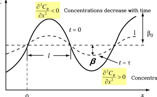
Ex1. Homogenization

of sinusoidal varying composition

in the elimination of segregation in casting

l : half wavelength

l C x

C = + β

sin π

: the mean composition C 　

0

: the amplitude of the initial concentration profile β

Initial or Boundary Cond.?

at t=0

2 0

2 >

∂

∂ x C_B

2 0

2 <

∂

∂ x C_B

Fig. 2.10 The effect of diffusion on a sinusoidal variation of composition.

Concentrations decrease with time

Concentrations increase with time.

∂ = ∂

∂ ∂

2 2

B B

B

C C

t D x

7

Rigorous solution of for

2 2

x D C t

C

∂

= ∂

∂

∂ ( )

l C x

x

C , 0 = + β

sin π

( )

( )

D l

t n

n

n n

n n

Dt

l e C x

C

A B

C A

l C x

C t

x B

x A

A C

e x B

x A

C

2 2

2

/ 0

0 1

0

0 1

0

sin , 0 ,

;

sin 0

cos sin

sin cos

π

λ

β π

β β π

λ λ

λ λ

−

∞

=

−

+

≡

∴

=

=

=

+

≡

→

=

+ +

=

∴

+

=

∴

∑

(A

= 0 for all others)

τ : relaxation time

 

 

 +  −

= τ

β π t

l C x

C

sin exp

D l

2 2

τ = π

) 2 /

0

exp(

x l at

t =

−

= β τ

β

2 2

2 2 2

1 1

Let

λ

−

≡

=

=

=

dx X d X dt

dT DT

dx X DT d

dt X dT

XT C

x B

x A

X dx X

X d

λ λ

λ

sin cos

2

0

2 2

+ ′

= ′

= +

Using a method of variable separation

l C β sin π x X(x,0) ≡ +

e

T T

dt D T d

dt D dT T

2

0

2 2

ln 1

λ

λ λ

=

−

=

−

=

l λ =π

8

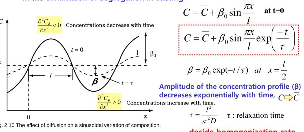
Solutions to the diffusion equations

Ex1. Homogenization of sinusoidal varying composition in the elimination of segregation in casting

l C x

C = + β

sin π at t=0

τ : relaxation time

 

 

 +  −

= τ

β π t

l C x

C

sin exp

D l

2 2

τ = π

) 2 /

0

exp(

x l at

t =

−

= β τ

β

The initial concentration profile will not usually be sinusoidal, but in general any con- centration profile can be considered as the sum of an infinite series of sine waves of varying wavelength and amplitude, and each wave decays at a rate determined by its

own “τ”. Thus, the short wavelength terms die away very rapidly and the homogenization will ultimately be determined by τ for the longest wavelength component.

decide homogenization rate

Fig. 2.10 The effect of diffusion on a sinusoidal variation of composition.

Amplitude of the concentration profile (β) decreases exponentially with time,

2 0

2 >

∂

∂ x C_B

2 0

2 <

∂

∂ x C_B

Concentrations decrease with time

Concentrations increase with time.

9

Solutions to the diffusion equations

Ex2. Carburization of Steel

The aim of carburization is to increase the carbon concentration in the surface layers of a steel product in order to achiever a harder wear-resistant surface.

1. Holding the steel in CH

and/or Co at an austenitic temperature.

2. By controlling gases the concentration of C at the surface of the steel can be maintained at a suitable constant value.

3. At the same time carbon continually

diffuses from the surface into the steel.

10

Carburizing of steel

The error function solution:

( ) ( ) 0 , , t C

C

C t

C

B

s B

=

∞

=

( )

( ) Ζ = ∫

 

 



− 

−

=

0 0

2

2 dy e

erf

Dt erf x

C C

C C

y s

s

π

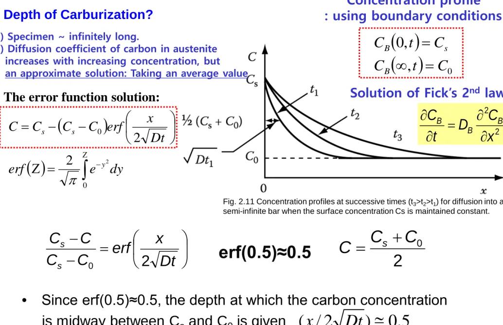
Depth of Carburization?

• Since erf(0.5)≈0.5, the depth at which the carbon concentration is midway between C

and C

is given

that is

( / 2 x Dt ) ≅ 0.5 x ≅ Dt

erf(0.5)≈0.5

 

 



= 

−

−

Dt erf x

C C

C C

s s

0

2

0

2 C

C

C +

=

→ Depth of Carburization

* Concentration profile : using boundary conditions

Solution of Fick’s 2

law

1) Specimen ~ infinitely long.

2) Diffusion coefficient of carbon in austenite increases with increasing concentration, but

an approximate solution: Taking an average value

Fig. 2.11 Concentration profiles at successive times (t₃>t₂>t₁) for diffusion into a semi-infinite bar when the surface concentration Cs is maintained constant.

∂ ∂

∂ = ∂

2 2

B B

B

C C

t D x

11

Error function

In mathematics, the error function (also called the Gauss error

function) is a non-elementary function which occurs in probability, statistics and partial differential equations.

It is defined as:

By expanding the right-hand side in a Taylor series and integrating, one can express it in the form

for every real number x. ( From Wikipedia, the free encyclopedia )

12

Error function = −

π ∫ O Z 2

erf(z) 2 exp( y )dy

Schematic diagram illustrating the main features of the error function.

13

Carburizing of steel

The error function solution:

( ) ( ) 0 , , t C

C

C t

C

B

s B

=

∞

=

( )

( ) Ζ = ∫

 

 



− 

−

=

0 0

2

2 dy e

erf

Dt erf x

C C

C C

y s

s

π

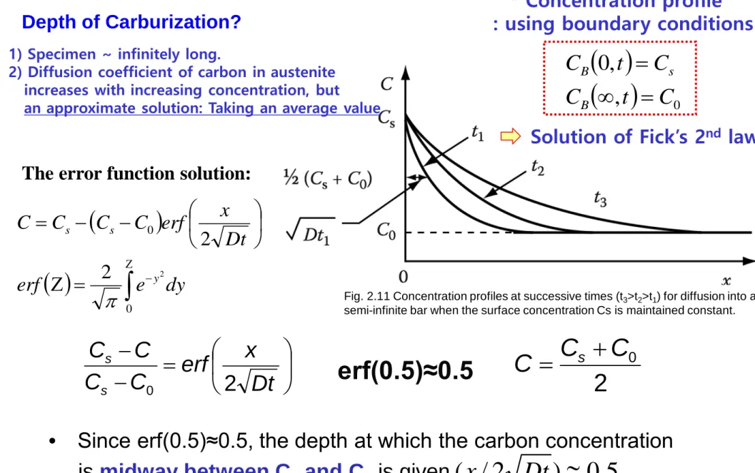
Depth of Carburization?

• Since erf(0.5)≈0.5, the depth at which the carbon concentration is midway between C

and C

is given

that is

( / 2 x Dt ) ≅ 0.5 x ≅ Dt

erf(0.5)≈0.5

 

 



= 

−

−

Dt erf x

C C

C C

s s

0

2

0

2 C

C

C +

=

→ Depth of Carburization

* Concentration profile : using boundary conditions

Solution of Fick’s 2

law

1) Specimen ~ infinitely long.

2) Diffusion coefficient of carbon in austenite increases with increasing concentration, but

an approximate solution: Taking an average value

Fig. 2.11 Concentration profiles at successive times (t₃>t₂>t₁) for diffusion into a semi-infinite bar when the surface concentration Cs is maintained constant.

14

Carburizing of steel

 

 



= 

Dt erf x

C

C

2

≅ Dt

Dt

Thus the thickness of the carburized layer is .

Note also that the depth of any is concentration line is directly proportion to , i.e. to obtain a twofold increase

in penetration requires a fourfold increase in time.

(2배의 침투 깊이 → 4배의 시간)

Ex.3 Decarburization of Steel?

( )

( ) Ζ = ∫

 

 



− 

−

=

0 0

2

2 dy e

erf

Dt erf x

C C

C C

y s

s

π

C

= Surface concentration C

= Initial bulk concentration

Carburization

15

= = −∞ < <

= = < < ∞

= = −∞ < < ∞

= = ∞ < < ∞

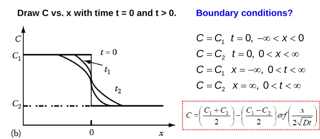
1 2 1 2

0, 0

0, 0 , 0 , 0

C C t x

C C t x

C C x t

C C x t

Joining of two semi-infinite specimens of compositions C

and C

(C

> C

) Draw C vs. x with time t = 0 and t > 0. Boundary conditions?

Solutions to the diffusion equations

Ex4. Diffusion Couple

Fig. 2.12 (b) concentration profiles at successive times (t2>t1>0)

when two semi-infinite bars of different composition are annealed after welding.

16

The section is completed with 4 example solutions to Fick's 2nd law:

carburisation, decarburisation, diffusion across a couple and homogenisation.

The solutions given are as follows:

l

Process Solution

Homogenization

C_mean = Mean concentration

b₀ = Initial concentration amplitude l = half-wavelength of cells

t = relaxation time

Carburization

C_S = Surface concentration C₀ = Initial bulk concentration

Decarburization

C₀ = Initial bulk concentration

Diffusion Couple

C₁ = Concentration of steel 1 C₂ = Concentration of steel 2

17

Q. Interstitial diffusion vs Substitutional diffusion

1. Self diffusion in pure material 2. Vacancy diffusion

3. Diffusion in substitutional alloys

1. Self diffusion in pure material

Probability of vacancy x probability of jump

• Interstitial Diffusion / Substitutional Diffusion

- Diffusion in dilute interstitial alloys ~ relatively simple

because the diffusing atoms are always surrounded by vacant sites to which they can jump whenever they have enough to overcome the energy barrier for migration.

- In substitutional diffusion,

An atom can only jump if there happens to be vacant site at one of the adjacent lattice positions

The rate of self-diffusion can be measured experimentally by intro- ducing a few radioactive A atoms (A*) into pure A and measuring the rate at which penetration occurs at various temperatures.

Since A* and A atoms are chemically identical their jump frequencies are almost identical.

1

A

6

D = Γ α

amenable to a simple atomic model: self-diffusion (순금속의 자기확산)

D

* =

Assumption

: unrelated to the previous jump

most likely to occur back into the same vacancy

D

* = f D

f

The next jump is not equally probable in all directions.

19

Q. Interstitial diffusion vs Substitutional diffusion

1. Self diffusion in pure material 2. Vacancy diffusion

3. Diffusion in substitutional alloys

20

Substitutional diffusion

1. Self diffusion in pure material

What would be the jump frequency in substitutional diffusion?

An atom next to a vacancy can make a jump provided it has enough thermal energy to overcome ∆G

.

The probability that an adjacent site is vacant → zX

→ exp( -∆G

/kT) Probability of vacancy x probability of jump

→ Γ = ν

−∆ G

zX exp

RT

=

= −∆ G

X X exp

RT

1

A

6

D = Γ α

= α ν 1

− ∆ ( G

+ ∆ G )

D z exp

6 RT

For most metals: ν ~ 10

, fcc metals : z = 12, α = a 2

G

cf ) z exp for int erstitials RT

Γ = ν −∆

Z=number of nearest neighbors/ ν= temperature independent frequency Jump frequency

In thermodynamic equilibrium, Z= # of nearest neighbours

21

)

0

exp(

RT D Q

D

= −

− ∆ + ∆

= α ν

A

1 ( G G )

D z exp

6 RT

For most metals: ν ~ 10

, fcc metals : z = 12, α = a 2 S T H

G = ∆ − ∆

∆

) exp(

6 exp 1

RT H H

R S z S

D

∆

+ ∆

∆ − +

= α ν ∆

R S z S

D ∆

+ ∆

= exp

6 1

0

α ν

V m

SD

H H

Q = ∆ + ∆

Z=number of nearest neighbors/ ν= temperature independent frequency

~Same with interstitial diffusion except that the activation energy for self-diffusion has an extra term

∵ self-diffusion requires the presence of vacancies

22

0 exp ID

B B

D D Q

RT

= −

m m m

G H T S

∆ = ∆ − ∆ 1

B

6

D = Γ α

B

? jump frequency Γ

Thermally activated process

Ζ : nearest neighbor sites ν : vibration frequency

∆G

: activation energy for moving

( ) ( )

ID m

m m

B

Q H

RT H

R S

D

≡

∆

∆

 −

 

 Ζ ∆

= exp / exp /

6

1 α

ν

( G

RT )

B

= Ζ exp − ∆ /

Γ ν

* interstitial diffusion

23

 

 



− 

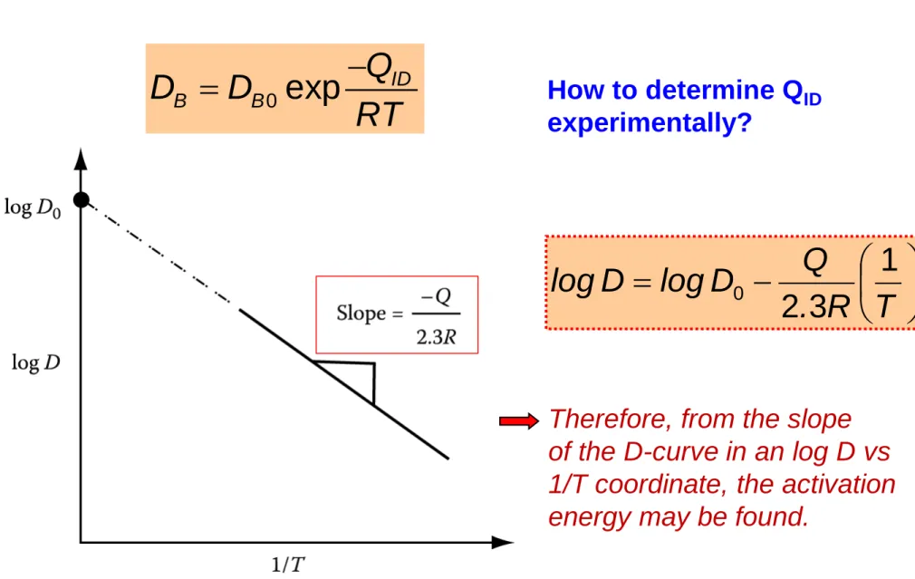
= . R T

D Q log D

log 1

3

0

2

Temperature Dependence of Diffusion

=

exp −

B B

D D Q

RT

Therefore, from the slope of the D-curve in an log D vs 1/T coordinate, the activation energy may be found.

How to determine Q

experimentally?

Fig. 2.7 The slope of log D v. 1/T gives the activation energy for diffusion Q.

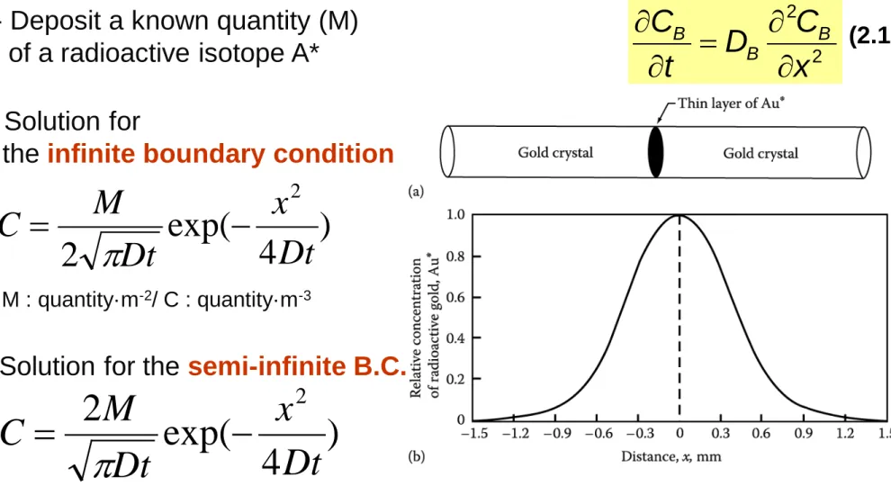
Fig. 2.14 Illustration of the principle of tracer diffusion and of the planar source method for determining the self-diffusion coefficient of gold. (a) Initial diffusion couple with planar source of radioactive gold Au*.

(b) Distribution of Au* after diffusion for 100h at 920℃

Experimental Determination of D

∂ ∂

∂ = ∂

2 2

B B

B

C C

t D x

1) Solution for

the infinite boundary condition

M : quantity·m

/ C : quantity·m

- Deposit a known quantity (M) of a radioactive isotope A*

4 ) 2 exp(

2

Dt x Dt

C = M −

π

4 )

2 exp( 2

Dt x Dt

C = M −

π

2) Solution for the semi-infinite B.C.

24

(2.18)

25

For a given structure and bond type, Q/RT

is roughly constant;

Q is roughly proportional to T

.

ex) for fcc and hcp, Q/RT

~ 18 and D(T

) ~ 1 µm

s

(10

m

s

)

For a given structure and bond type, D(T/T

) ~ constant

T/T

: homologous temperature

Within each class, D(T

) and D

are approximately constants.

Most close-packed metals Table 2.2 Experimental Data for Substitutional Self-Diffusion

in Pure Metals at Atmospheric Pressure

26

* Melting point diffusivities for various classes of materials:

: The diffusion coefficients of all materials with a given crystal structure and bond type will be approximately the same at the same fraction of their melting temperature, i.e. D(T/T_m) = const.

: Since volume usually increases on melting (T_m), raising the pressure increases T_m and thereby lowers the diffusivity at a given temperature.

1. Within each class, D(T

) ~ approximately constants.

27 : Q and T_m exhibit rough linear correlation because increasing the interatomic bond strength makes the process of melting more difficult; that is, T_m is raised.

It also makes diffusion more difficult by increasing ΔH_m & ΔH_v.

For a given structure and bond type, Q/RT

is roughly constant;

< Relationship between latent heat and melting point>

b) A

~ 1 for all liquid, A

depends on crystal structure

- Metallic structure (FCC, C.P.H, and BCC, “less localized bonding”) ~ good relationship compared with the structures which are covalently bonded (“specific directional bonds”) . - Molecular liquid such as F

, Cl

~ extra condition for A

( molecule must be correctly oriented in order to be accommodated.)

29

ex) At 800

C, D

= 5 × 10

mm

s

, α = 0.25 nm

2

6

1

α

D

= Γ Γ

= 5 × 10

jumps s

After an hour, diffusion distance (x)? Dt ~ 4 µ m

Cu : ? Γ

At 20

C, D

~ 10

mm

s

Γ

~ 10

jumps s

→ Each atom would make one jump every 10

years!

Hint) From the data in Table 2.2, how do we estimate D

at 20

C?

How do we determine D

at low temperature such as 20

C?

Consider the effect of temperature on self-diffusion in Cu:

Fig. 2.7 The slope of log D v. 1/T gives the activation energy for diffusion Q.

30

Q. Interstitial diffusion vs Substitutional diffusion

1. Self diffusion in pure material 2. Vacancy diffusion

3. Diffusion in substitutional alloys

31

All the surrounding atoms are possible

jump sites of a vacancy, which is analogous to interstitial diffusion.

) /

exp(

) / 6 exp(

1 6 1

2 2

RT H

R S

zv D

m m

v v

∆

−

∆

=

Γ

=

α α

Comparing D

with the self-diffusion coefficient of A, D

, 2. Vacancy diffusion

e v A

v

D X

D = /

This shows in fact that the diffusivity of vacancy (D

) is many orders

of magnitude greater than the diffusivity of substitutional atoms (D

).

32

3. Diffusion in substitutional alloys

J

J

J

At t = 0 ,

At t = t

,

J

J

J

’

J

J

J

’ x D C J

J

J

∂

− ∂

= +

′ = ~

x D C J

J

J

∂

− ∂

= +

′ = ~

B A A

B

D X D

X

D ~ = +

 

 





∂

∂

∂

= ∂

∂

∂

x D C x t

C

~

A

B

J

J ′ = − ′

∴

* During self-diffusion, all atoms are chemically identical

: probability of finding a vacancy and jumping into the vacancy ~ equal

* In binary substitutional alloys, each atomic species must be

given its own intrinsic diffusion coefficient D

or D

.

33

3. Diffusion in substitutional alloys

J

J

J

At t = 0 ,

At t = t

,

J

J

J

’

J

J

J

’ x D C vC

J J

J

J

∂

− ∂

= +

= +

′ = ~

x D C vC

J J

J

J

∂

− ∂

= +

= +

′ = ~

B A A

B

D X D

X

D ~ = +

 

 





∂

∂

∂

= ∂

∂

∂

x D C x t

C

~

A

B

J

J ′ = − ′

A원자와 B원자가 서로 다른 속도로 도약 → ∴

농도 구배에 의한 속도 + 격자면 이동에 의한 속도

A-rich AB B-rich AB 확산이 일어나는 격자이동에 의한 A 유속

공공의 net flux

침입형 확산에서 Fick의 법칙 고정된 격자면을 통한 이동 : A원자/B원자의 상호확산을 통한 격자면의 이동 고려

확산이 일어나는 격자이동에 의한 B 유속 고정된 격자 내에서 확산에 의한 유속

고정된 격자 내에서 확산에 의한 유속