Byeng D. Youn
System Health & Risk Management Laboratory Department of Mechanical & Aerospace Engineering Seoul National University
Chapter 3. Energy Methods
1
WorkCastigliano’s Theorem
2
Example
3
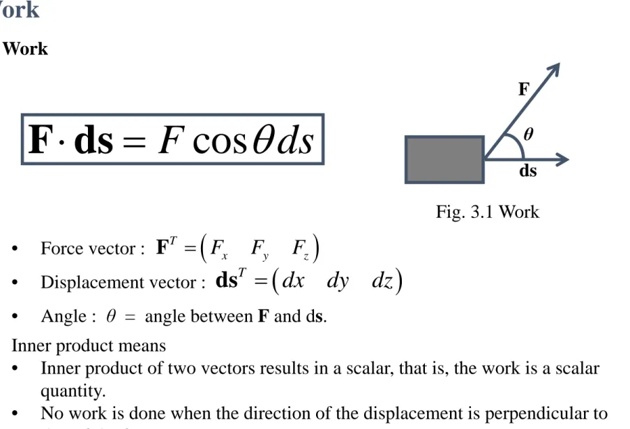
Work
Work
Inner product means
• Inner product of two vectors results in a scalar, that is, the work is a scalar quantity.
• No work is done when the direction of the displacement is perpendicular to that of the force.
• Force vector :
• Displacement vector :
• Angle : θ = angle between F and ds.
( )
T
x y z
F F F
=
F ds
T= ( dx dy dz )
cos
F θ ds
⋅ = F ds
F
ds θ
Fig. 3.1 Work
Work
General Work
There are two kinds of work.
• Conservative: work done by external force is stored in the form of potential energy, and recoverable.
(ex. gravitational potential energy, elastic potential energy)
• Non-conservative: work done in system is not recoverable.
(ex. sliding block with friction)
( ) ⋅
∫ F s ds
We use general work when force varies with a point of application.
a
b
F ds θ
Fig. 3.2 General Work
Work
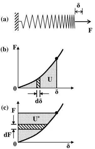
General Work (Elastic Spring)
• The general work is stored in the form of a potential energy.
• The potential energy appears as the shaded area in Fig. 3.1 (b).
• U (potential energy) is a function of elongation δ.
F (external force) remains in equilibrium with the internal tension (spring force = kδ).
*
0
Fd U
δ
δ
⋅ = =
∫ F ds ∫
Fig. 3.1 Nonlinear spring undergoes a gradual elongation.
δ F
dδ U 0
(b)
F
dF
U*
0 δ
(c) (a)
δ F
Work
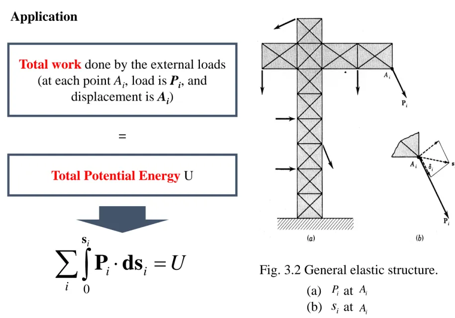
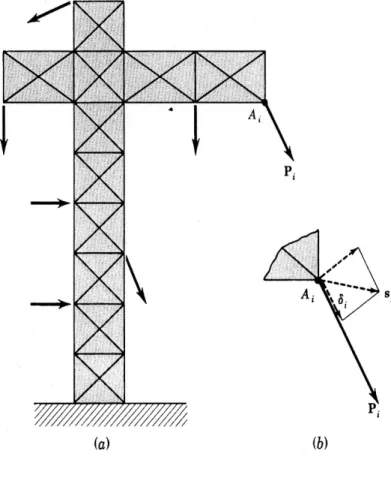
Application
Fig. 3.2 General elastic structure.
(a) at (b) at
Pi Ai
si Ai
Total work done by the external loads (at each point Ai, load is Pi, and
displacement is Ai)
=
Total Potential Energy U
0
i
i i
i
⋅ = U
∑∫
sP ds
Work
Complementary Work
• This energy appears as the shaded area in Fig. 3.1 (c)
• U* (complementary energy) is a function of the force F.
When complementary work is done on this system, their internal force states alter in such a way that they are capable of giving up equal amounts of complementary work when they are returned to their original force states. Under these circumstances the complementary work done on such system is said to be stored as complementary energy.
0
*
F
dF U
δ
⋅ = =
∫ s dF ∫
Fig. 3.1 Nonlinear spring undergoes a gradual elongation.
δ F
dδ U 0
(b)
F
dF
U*
0 δ
(c) (a)
δ F
Work
Application
Fig. 3.2 General elastic structure.
(a) at (b) at
Pi Ai
si Ai
Total complementary work done by the external loads
(at each point Ai, load is Pi, and displacement is Ai)
=
Total Complementary Energy U*
0 0
*
i Pi
i i i i
i i
dP U δ
⋅ = =
∑
P∫ s dP ∑ ∫
where si can be decomposed into parallel and perpendicular to . The parallel component is δ i. (Fig. 3.2b)
si
P
iδ
iCastigliano’s Theorem
Fig. 3.2 General elastic structure.
(a) at (b) at
Pi Ai
si Ai
Now if the loads in Fig. 3.2 (a) are
gradually increased from zero so that the system passes through a succession of
equilibrium states, the total complementary work done by all the external loads will equal the total complementary energy U*
stored in all the internal elastic members.
Let’s consider a small increment ∆Pi
i i
i i
P U or
U P
δ δ
∆ =
∆
∆
=
∆
*
*
Castigliano’s Theorem
In the limit as →0 this approaches a derivative which we indicates as a partial derivative since all other loads were held fixed. is a in-line deflection.
This result is a form of Castigliano’s theorem.
Pi
∆
i
P
iU = δ
∂
∂ *
The theorem can be extended to include moment loads.
where is moment loads, and is an angle of rotation.
Mi
φ
i*
i i
U
M φ
∂ =
∂
δ
iCastigliano’s theorem in linear system
Castigliano’s Theorem
In nonlinear system U* ≠ U In linear system U* = U
δ F
dδ U 0
(b)
F
dF
U*
0 δ
(c) δ
F
0
F = kδ
U
δ F
0
F = kδ U*
Example : Linear spring (1)
Castigliano’s Theorem
k F F
k U
U U
k U F
k U
k F
2 2
1 2
1
*
* 2 2 ,
1
2 2
2 2
=
=
=
=
=
=
=
δ δ
δ δ
where k is spring constant
δ F
0
F = kδ
U
δ F
0
F = kδ U*
Example : Linear spring (2)
Castigliano’s Theorem
EA L P L
U EA L k EA
2 2
2 2
=
=
=
δ
For the linear uniaxial member in Figs. 3.3 and 3.4
EA PL EA
L P P
P U
i i
i
=
∂
= ∂
∂
= ∂
2 δ
2Finally, the in-line deflection at any loading point is obtained by differentiation of the potential energy with respect to the load
Ai
δ
iL1+ δ1
L1
P A1 P
L2+ δ2
L2 = L1
P A2 P
L3+ δ3
L3
P A3 = A2 P
δ P
0
Linear material
1 2 3
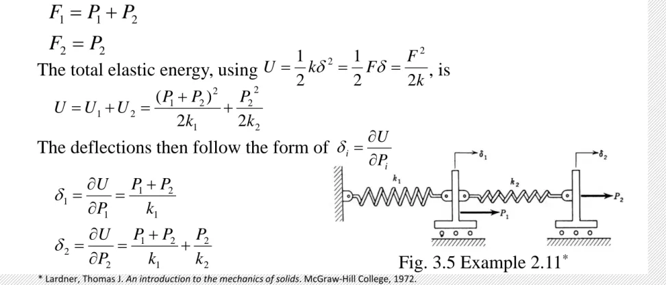
Fig. 3.5 Example 2.11* Example 1*
Castigliano’s Theorem
Consider the system of two springs shown in Fig. 3.5. We shall use Castigliano’s theorem to obtain the deflections and which are due to the external loads
and .
To satisfy the equilibrium requirements the internal spring forces must be
The total elastic energy, using , is
The deflections then follow the form of
δ
1δ
2P1 P2
2 2
2 1
1
P F
P P
F
= +
=
k F F
k
U 2 2
1 2
1 2 = = 2
= δ δ
2 2 2 1
2 2 1 2
1 2 2
) (
k P k
P U P
U
U = + = + +
2 2 1
2 1 2
2
1 2 1 1
1
k P k
P P P
U
k P P P U
+ +
∂ =
= ∂
= +
∂
= ∂ δ δ
i
i P
U
∂
= ∂ δ
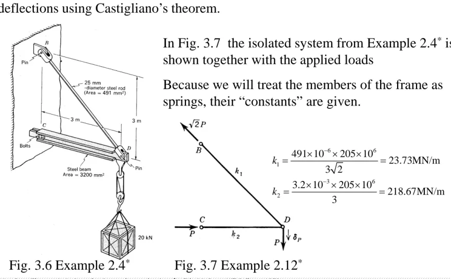
Example 2*
Castigliano’s Theorem
Let us consider again Example 2.4* (also Example 1.3*), and determine the deflections using Castigliano’s theorem.
Fig. 3.6 Example 2.4*
In Fig. 3.7 the isolated system from Example 2.4* is shown together with the applied loads
Because we will treat the members of the frame as springs, their “constants” are given.
Fig. 3.7 Example 2.12*
6 6
1
3 6
2
491 10 205 10
23.73MN/m 3 2
3.2 10 205 10
218.67MN/m 3
k
k
−
−
× × ×
= =
× × ×
= =
Example 2* (Continued)
Castigliano’s Theorem
We use the equilibrium requirements to express the member forces and in terms of the load P so that the total energy is
We can calculate directly the deflection of point D from
F1 F2
2 2
1 2
2 2 2 1
2 1 2
1
2 2 2 k
P k
P k
P k
U P U
U = + = + = +
i
i P
U
∂
= ∂ δ
( )
2 2
1
1 2 2
3 6
1
1 1
2
2 2
2 20 10 0.0421 0.0023 10 1.77mm
P
U P P
P
P P k k k k
δ
δ
−∂ ∂
= = + = +
∂ ∂
= × × × + × =
In order to calculate the horizontal deflection at point D using Castigliano’s theorem, there must be a horizontal force at D. But the horizontal force at D is zero.
We can satisfy both requirements by applying a fictitious horizontal force Q and setting Q = 0.
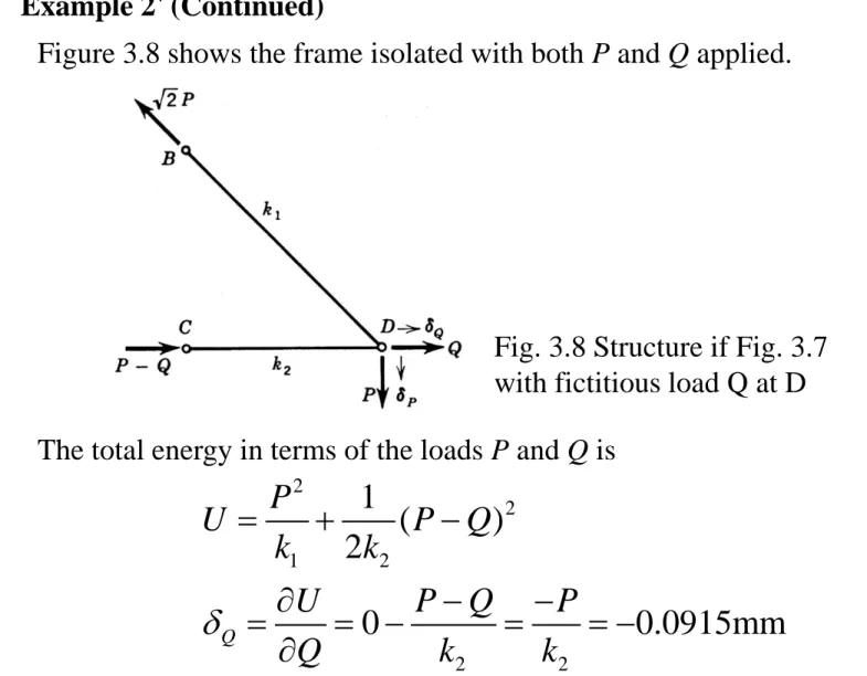
Example 2* (Continued)
Castigliano’s Theorem
Figure 3.8 shows the frame isolated with both P and Q applied.
The total energy in terms of the loads P and Q is
2
2
1 2
2 2
1 ( )
2
0 0.0915mm
Q
U P P Q
k k
U P Q P
Q k k
δ
= + −
∂ − −
= = − = = −
∂
Fig. 3.8 Structure if Fig. 3.7 with fictitious load Q at D
Example 3*
Castigliano’s Theorem
Let us use Castigliano’s theorem to determine deflections in the Truss problem that we considered in Example 2.5* and in the computer solution example of Sec.
2.5*.
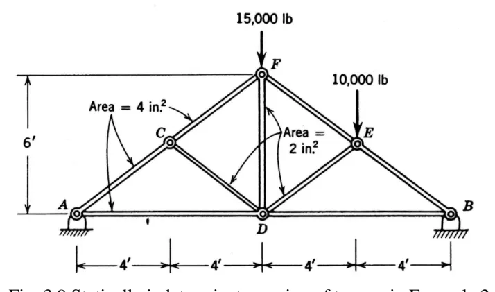
Fig. 3.9 Statically indeterminate version of trusses in Example 2.5*.
Example 3* (Continued)
Castigliano’s Theorem
If a truss is made of n axially loaded members,
(energy stored in the i th member)
(total energy in the system of n members)
2
1
2
i i
i
i i
n i i
U F L
A E
U U
=
=
= ∑
The deflection at any external load P in the direction of P, is
∂ =
= ∂
∂
= ∂
∂
= ∂ ∑ ∑
=
=
P
F E A
L F E
A L F P
P
U
n ii i i
i i n
i i i
i i P
1 1
2
δ 2
P F E
A
F L
in
i i i
i
i
∂
∑ ∂
=1
(a)
Example 3* (Continued)
Castigliano’s Theorem
We will number the members as shown in Fig. 3.10.
In example 2 we solved for the forces due to the actual applied loads.
We can now set up a system for evaluating (a).
The deflection at the joint at which the fictitious load P is applied, it appears that we need to find the forces in each members as a function of the actual applied loads and fictitious load P.
However, once the member forces are found, we set P = 0 in (a).
Therefore, we can use immediately the member forces from the actual loads and the forces for a unit load at P to evaluate .
Fig. 3.10 Example 2.13*.
P F
i∂
∂ / F
iF
iF
iExample 3* (Continued)
Castigliano’s Theorem
In the Table 3.1 we have tabulated the individual quantities in (a) as well as their products.
Table 3.1 Truss solution by energy methods
Example 3* (Continued)
Castigliano’s Theorem
If we wish to solve for the deflection at P, we must reevaluate the products in row 1 and 2 of Table 3.1 with Q.
The values for member 3 through 9 do not change since they carry no Q.
Therefore
10
62 . 3 1651 .
0 + ×
−∂ =
= ∂ Q
P U
δ
P hereQ = − 16 . 67 × 10
30.1651 0.0534 0.1117in δ
P∴ = − =
Rotation of Axes, etc
It can be seen that the second order tensor map a vector to another vector, that is,
Symmetric Tensor
11 1 1 12 1 2 13 1 3
21 2 1 22 2 2 23 2 3
31 3 1 32 3 2 33 3 3 1 1 2 2 3 3
11 1 12 2 13 3 1 21 1 2
(
) ( )
= ( ) (
T T T T
T T T
T T T v v v
T v T v T v T v T
= ⋅ = ⊗ + ⊗ + ⊗
+ ⊗ + ⊗ + ⊗
+ ⊗ + ⊗ + ⊗ ⋅ + +
+ + + +
u v e e e e e e
e e e e e e
e e e e e e e e e
e 2 2 23 3 2
31 1 32 2 33 3 3
)
( )
ij j i
v T v T v T v T v
T v
+
+ + +
=
e e
e
Symmetric tensors and skew tensors
Skew or Antisymmetric Tensor
ji
ij T
T =
ji
ij T
T = −
THANK YOU
FOR LISTENING