Trees
Introduction to Data Structures Kyuseok Shim
SoEECS, SNU.
5.1 Introduction
5.1.1 Terminology
Tree : a finite set of one or more nodes
there is a specially designated node called the root
the remaining nodes are partitioned into n≥0 disjoin t sets T
1, ..., T
n, where each of these sets is a tree.
T
1, ..., T
nare called the subtrees of the root.
Degree of a node : the number of subtrees of a node
Leaf (terminal node) : a node that has degree zero
Nonterminals : the other nodes
Children, parent, siblings
5.1.1 Terminology
Degree of a tree : the maximum of degree of th e nodes in the tree
Ancestors of a node : all the nodes along the p ath from the root to that node
Level of a node : the distance from the root+1
Height (or depth) of a tree : the maximum level
of any node in the tree
Dusty
Honey Bear
Brungilde
Gill Tansey
Terry
Tweed Zoe
Brandy
Coyote
Crocus Primrose
Nugget
Nous Belle
5.1.1 Terminology
Proto Indo-European
Italic
Osco- Umbrian
Oscan Umbrian
Latin
Spanish French Italian
Hellenic
Greek
Germanic
North
Iceland Norwegian Swedish
West
Low High Yiddish
(a) Pedigree
(b) Lineal
5.1.1 Terminology
A
B
E F
D
H J
K L
level 1
2
3
4 C
G I
M
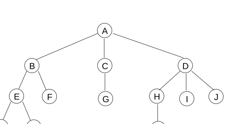
Figure 5.2 : A sample tree
5.1.2 Representation of Trees
List representation
The tree of Figure 5.2
(A(B(E(K,L),F),C(G),D(H(M),I,J)))
The degree of each node may be different
possible to use memory nodes with a varying number of pointer fields
easier to write algorithms when the node
size is fixed
5.1.2 Representation of Trees
List representation
nodes of a fixed size
for a tree of degree k
Lemma 5.1: If T is a k-ary tree with n nodes, each ha ving a fixed size, then n(k-1)+1 of the nk child fields are 0, n≥1.
Proof: Since each non-zero child field points to a node and there is exactly one pointer to each node other than the root, the number of child fields in a k-ary tree with n nodes is nk. Hence, the number of zero fields is nk – (n-1) = n(k-1)+1
DATA CHILD1 CHILD2 ⋯ CHILDk
5.1.2 Representation of Trees
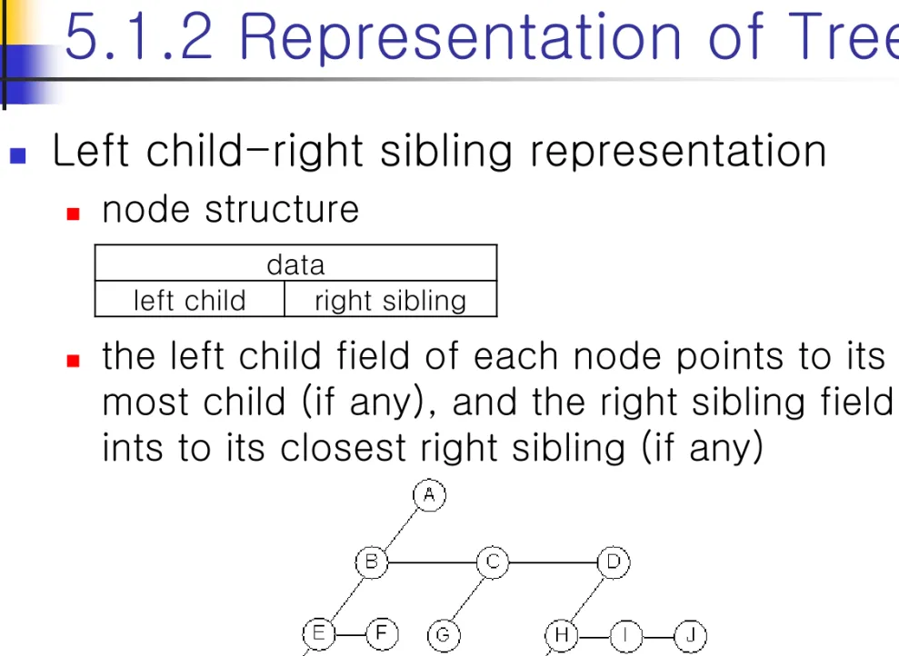
Left child-right sibling representation
node structure
the left child field of each node points to its left most child (if any), and the right sibling field po ints to its closest right sibling (if any)
data
left child right sibling
Figure 5.6 : Left child-right sibling representation of the tree of Figure 5.2
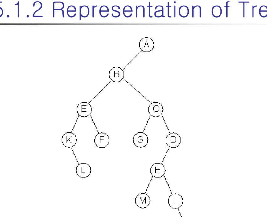
5.1.2 Representation of Trees
Representation as a degree-two tree
rotate the right-sibling pointers clockwis e by 45 degrees
the two children of a node are referred t o as the left and right children
A
B B
5.1.2 Representation of Trees
Figure 5.7 : Left child-right child tree representation
5.1.2 Representation of Trees
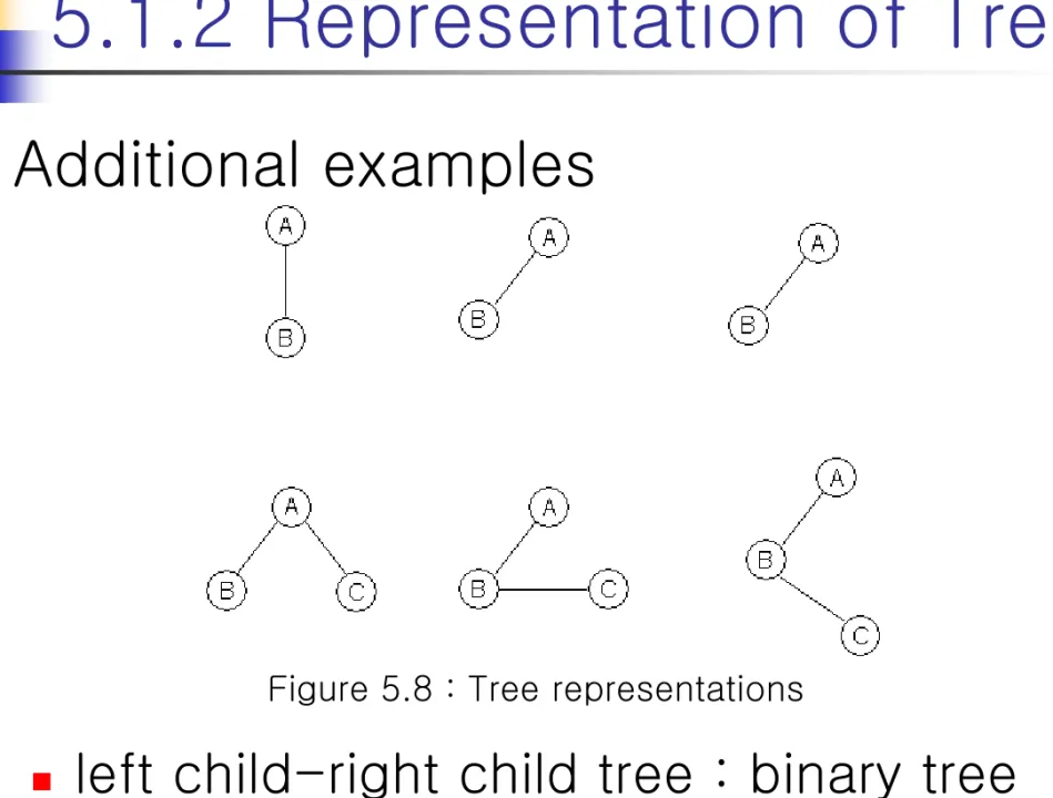
Additional examples
left child-right child tree : binary tree
any tree can be represented as a binary tree
Figure 5.8 : Tree representations
5.2 Binary Trees
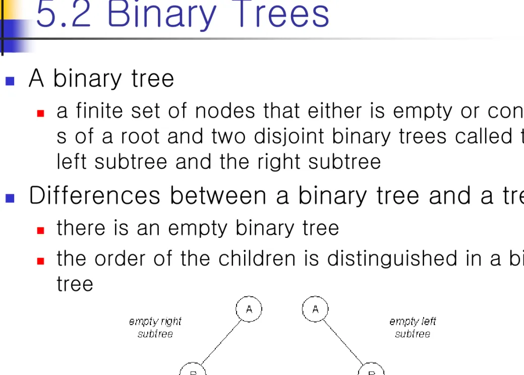
A binary tree
a finite set of nodes that either is empty or consist s of a root and two disjoint binary trees called the left subtree and the right subtree
Differences between a binary tree and a tree
there is an empty binary tree
the order of the children is distinguished in a binary tree
Figure 5.9 : Two different binary trees
5.2 Binary Trees
template <class T>
class BinaryTree
{ // objects: A finite set of nodes either empty or consisting of a // root node, left BinaryTree and right BinaryTree.
public:
BinaryTree();
// creates an empty binary tree bool IsEmpty();
// return true if the binary tree is empty
BinaryTree(BinaryTree<T>& bt1, T& item, BinaryTree<T>& bt2);
// creates a binary tree whose left subtree is bt 1, whose right // subtree is bt 2, and whose root node contains item
BinaryTree<T> LeftSubtree();
// return the left subtree of *this BinaryTree<T> RightSubtree();
// return the right subtree of *this T RootData();
// return the data in root node of *this };
--- ADT 5.1 : Abstract data type BinaryTree
5.2 Binary Trees
A
B
D E
C
F G
H I
A B
C
D
E
level 1
2
3
4 5
(a) (b)
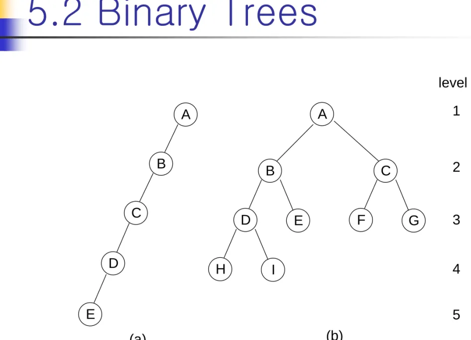
Figure 5.10 : Skewed and complete binary trees
5.2.2 Properties of Binary Trees
Lemma 5.2 [Maximum number of nodes]:
(1) The max number of nodes on level i of a binary tree is 2
i-1, i≥1
(2) The max number of nodes in a binary tree o
f depth k is 2
k-1, k≥1
5.2.2 Properties of Binary Trees
Proof:
(1) The proof is by induction on i.
Induction Base : The root is the only node on level i = 1.
Hence, the maximum number of nodes on level i = 1 is 2i-1=20=1
Induction Hypothesis : Let i be an arbitrary positive integer greater than 1.
Assume that the maximum number of nodes on level i-1 is 2i-2
Induction Step : The maximum number of nodes on level i-1 is 2i-2 by the induction hypothesis. Since each node in a binary tree has a maximum degree of 2, the maximum number of nodes on level i is two times the maximum number of nodes on level i-1, or 2i-1
(2) The maximum number of nodes in a binary tree of depth k is
1 2 2
) (max
1 1
1 = −
∑
=∑
= =
− k
k
i
k
i
i i
level on
nodes of
number imum
5.2.2 Properties of Binary Trees
Lemma 5.3 [Relation between numbe r of leaf nodes and degree-2 nodes]:
For any non-empty binary tree, T,
if n 0 is the number of leaf nodes and
n 2 the number of nodes of degree 2,
then n 0 =n 2 +1
5.2.2 Properties of Binary Trees
Proof : Let n
1be the number of nodes of degree one and n the total number of nodes. Since all nodes in T are at most of degree two, we have n=n
0+n
1+n
2If we count the number of branches in a binary tree, we see that every node except the root has a branch leading into it. If B is the number of branches, then n=B+1. All branches stem from a node of degree one or two. Thus, B=n
1+2n
2. Hence,
we obtain n = B+1 = n
1+2n
2+1. We get n
0= n
2+ 1
Def : A full binary tree of depth k
a binary tree of depth k having 2
k-1 nodes, k≥0
5.2.2 Properties of Binary Trees
A binary tree with n nodes and depth k is complete
its nodes correspond to the nodes numbered from 1 to n in the full binary tree of depth k
The height of a complete binary tree with n nodes is
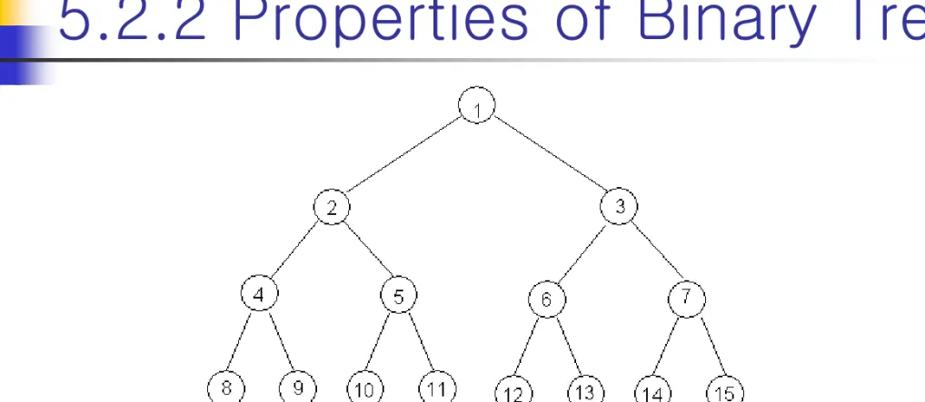
Figure 5.11 : Full binary tree of depth 4 with sequential node numbers
⎡
log2(n+1)⎤
5.2.3 Binary Tree Representation 5.2.3.1 Array Representations
Lemma 5.4 : If a complete binary tree
with n nodes is represented sequentially, then for any node with index i, 1≤i≤n,
we have
(1) parent(i) is at i/2 if i≠1. If i=1, i is at the r oot and has no parent
(2) leftChild(i) is at 2i if 2i≤n. If 2i>n, then i ha s no left child
(3) rightChild(i) is at 2i+1 if 2i+1≤n. If 2i+1>n,
then i has no right child
5.2.3 Binary Tree Representation 5.2.3.1 Array Representations
Proof : We prove (2). (3) is an immediate consequence of (2) and the numbering of nodes on the same level from left to right. (1) follows from (2) and (3). We prove (2) by induction on i.
For i=1, clearly the left child is at 2 unless 2>n, in which chase i has no left child. Now assume that for all j,
1≤j≤i, leftChild(j) is at 2j.
Then the two nodes immediately preceding leftChild(i+1) are the right and left children of i. The left child is at 2i.
Hence, the left child of i+1 is at 2i+2=2(i+1) unless
2(i+1)>n, in which case i+1 has no left child
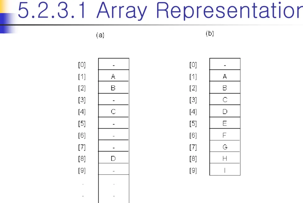
5.2.3.1 Array Representations
Figure 5.12 : Array representation of the binary trees of Figure 5.10
data
LeftChild RightChild
LeftChild data RightChild
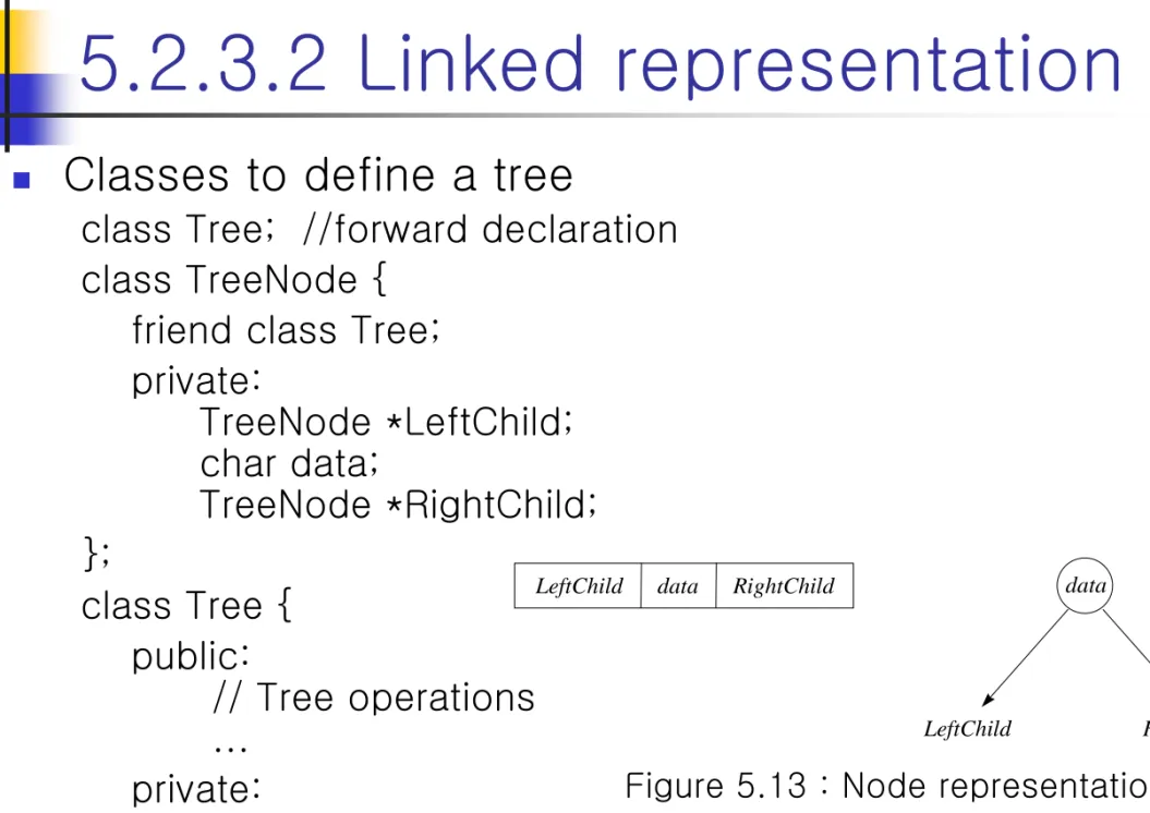
5.2.3.2 Linked representation
Classes to define a tree
class Tree; //forward declaration class TreeNode {
friend class Tree;
private:
TreeNode *LeftChild;
char data;
TreeNode *RightChild;
};
class Tree { public:
// Tree operations ...
private:
TreeNode *root;
};
Figure 5.13 : Node representations
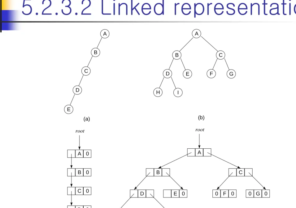
5.2.3.2 Linked representation
A
B
D E
C
F G
H I
A
B
C
D
E
(a) (b)
A 0
B 0
C 0
D 0
0 E 0 root
A root
B
E 0 D
0 H 0 0 I 0
C
0 G 0 0 F 0
Figure 5.14 : Linked representation for the binary trees of Figure 5.10
5.3 Binary Tree Traversal and Tree Iterators 5.3.1 Introduction
Tree traversal
visiting each node in the tree exactly once
a full traversal produces a linear order for the nodes
Order of node visit
L : move left V : visit node R : move right
possible combinations : LVR, LRV, VLR, VRL, RVL, RLV
traverse left before right
LVR : inorder
LRV : postorder
VLR : preorder
5.3.1 Introduction
+
∗
/
B
C A
D
E
∗
Figure 5.16 : Binary tree with arithmetic expression
5.3.2 Inorder Traversal
LVR
template<class T>
void Tree::inorder()
{ // Driver call workhorse for traversal of entire tree. The driver is // declared as a public member function of Tree.
inorder(root);
}
template<class T>
void Tree<T>::inorder(TreeNode<T> *CurrentNode)
{ // Workhorse traverses the subtree rooted at CurrentNode
// The workhorse is declared as a private member function of Tree.
if (CurrentNode) {
inorder(CurrentNode->leftChild);
Visit(currentNode);
inorder(CurrentNode->rightChild);
} }
--- Program 5.1 : Inorder traversal of a binary tree
※ Visit(TreeNode<T> *CurrentNode) { cout << currentNode->data
}
5.3.2 Inorder Traversal
Call of inorder
Value in
CurrentNode Action
Call of inorder
Value in
CurrentNode Action
Driver + 10 C
1 * 11 0
2 * 10 C cout<<'C'
3 / 12 0
4 A 1 * cout<<'*'
5 0 13 D
4 A cout<<'A' 14 0
6 0 13 D cout<<'D'
3 / cout<<'/' 15 0
7 B Driver + cout<<'+'
8 0 16 E
7 B cout<<'B' 17 0
9 0 16 E cout<<'E'
2 * cout<<'*' 18 0
Figure 5.17 : Trace of Program 5.1
Output : A/B*C*D+E
infix form of the expression
5.3.3 Preorder Traversal
VLR
template <class T>void Tree<T>::preorder() { // Driver
preorder(root);
}
template <class T>
void Tree<T>::preorder(TreeNode<T> *CurrentNode) { // Workhorse
if (CurrentNode) {
Visit(CurrentNode);
preorder(CurrentNode->leftChild);
preorder(CurrentNode->rightChild);
} }
--- Program 5.2 : Preorder traversal of a binary tree
∙ Output : +**/ABCDE
- prefix form of the expression
5.3.4 Postorder Traversal
LRV
template <class T>
void Tree<T>::Postorder() { // Driver
postorder(root);
}
template <class T>
void Tree::postorder(TreeNode *CurrentNode) { // Workhorse
if (CurrentNode) {
postorder(CurrentNode->LeftChild);
postorder(CurrentNode->RightChild);
Visit(currentNode);
} }
--- Program 5.3 : Postorder traversal of a binary tree
∙ Output : AB/C*D*E+
- postfix form of the expression
5.3.5 Iterative Inorder Traversal
Tree is a container class
may implement a tree traversal algorithm by using iterators
the algorithm needs to be non-recursive
use template Stack class
Definition
a data object of Type A USES-A data object of Type B if a Type A object uses a Type B object to perform a task
this relationship is typically expressed by emplo
ying the Type B object in a member function of
Type A
5.3.5 Iterative Inorder Traversal
template <class T>
void Tree<T>::NonrecInorder()
{ // nonrecursive inorder traversal using a stack
Stack<TreeNode<T> *> s; // declare and initialize stack TreeNode<T> *currentNode = root;
while(1) {
while(currentNode) { // move down LeftChild fields s.Push(currentNode); // add to stack
currentNode = currentNode->leftChild;
}
if (s.IsEmpty()) return;
currentNode = s.Top();
s.Pop();
Visit(currentNode);
currentNode = currentNode->rightChild;
} }
--- Program 5.4 : Nonrecursive inorder traversal
5.3.5 Iterative Inorder Traversal
class InorderIterator { public:
InorderIterator(){ CurrentNode = root;};
T* Next();
private:
Stack <TreeNode<T> *> s;
TreeNode<T>* currentNode;
};
--- Program 5.5 : Definition of inorder iterator class
T* InorderIterator::Next() {
while(currentNode) { s.Push(currentNode);
currentNode = currentNode->leftChild;
}
if (s.IsEmpty()) return 0;
currentNode = s.Top();
s.Pop();
T& temp = currentNode->data;
currentNode = currentNode->rightChild; // update return &temp;
}
--- Program 5.6 : Code for obtaining the next inorder element
5.3.6 Level-Order Traversal
Root-left child-right child
requires a queue
Output : +*E*D/CAB
used the circular queue
template <class T>
void Tree<T>::LevelOrder()
{ // Traverse the binary tree in level order Queue<TreeNode<T>*> q;
TreeNode<T> *currentNode = root;
while(currentNode) { Visit(currentNode);
if (currentNode->leftChild) q.Push(currentNode->leftChild);
if (currentNode->rightChild) q.Push(currentNode->rightChild);
currentNode = *q.Front();
q.Pop();
} }
--- Program 5.7 : Level-order traversal of a binary tree
5.3.7 Traversal without a Stack
Is binary tree traversal possible without the use of extra space for stack?
Add a parent field to each node
Another solution represents binary tree
as threaded binary trees in Section 5.5
5.4 Additional Binary Tree Operations 5.4.1 Copying Binary Trees
Implement a copy constructor
Using modified postorder traversal algorithm
Assume TreeNode has a constructor that sets all three data members of a tree
node
5.4.1 Copying Binary Trees
template <class T>
bool Tree<T>::Tree(const Tree<T>& s) //driver { // Copy constructor
root = Copy(s.root);
}
template <class T>
TreeNode<T>* Tree<T>::Copy(TreeNode<T>* origNode) // Workhorse
{ // Return a pointer to an exact copy of the binary tree rooted at origNode.
if(!origNode) return 0;
return new TreeNode<T>( origNode->data,
Copy(origNode->leftChild);
Copy(origNode->rightChild);
}
--- Program 5.9 : Copying a binary tree
5.4.2 Testing Equality
Determining the equivalence of two binary trees
They have the same topology and data in corresponding node is identical
Function operator==() calls workhorse
function Equal()
5.4.2 Testing Equality
template <class T>
bool Tree<T>::operator==(const Tree<T>& s) const//driver {
return Equal(root, t.root);
}
template <class T>
bool Tree<T>::Equal(TreeNode<T>* a, TreeNode<T>* b) {// Workhorse
if((!a)&&(!b)) return true; // both a and b are 0
return ( a&&b // both a and are non-zero
&& (a->data==b->data) // data is the same
&& Equal(a->leftChild, b->leftChild) // left subtrees equal
&& Equal(a->rightChild, b->rightChild)); // right subtrees equal }
--- Program 5.10 : Binary tree equivalence
5.4.3 The Satisfiability Problem
Consider the operations ∧(and),
∨(or), ¬(not)
The variables can hold only true or false
Example : x 1 ∨(x 2 ∧ ¬x 3 )
x
1=x
3=false, x
2=true
false ∨(true∧ ¬false)
= false∨true = true
Let assume our formula is
(x
1∧ ¬ x
2)∨(¬x
1∧ x
3)∨¬x
35.4.3 The Satisfiability Problem
∨
∨
∧
¬
¬
¬
∧ x1
x1 x2
x3
x3
Figure 5.18 : Propositional formula in a binary tree
5.4.3 The Satisfiability Problem
There are 2 n possible combination
if n=3, true=t, false=f
(t,t,t), (t,t,f), (t,f,t), (t,f,f), (f,t,t), (f,t,f) (f,f,t), (f,f,f)
O(2
n) time complexity
To evaluate an expression, using postorder traversal
(x
1∧ ¬ x
2)∨(¬x
1∧ x
3)∨¬x
3=> x
2¬x
1∧x
1¬ x
3∧∨x
3¬∨
5.4.3 The Satisfiability Problem
Define new data type
T = pair<Operator, bool>
enum Operator{Not, And, Or, True, False}
Program 5.11
n is the number of variables in formula
formula is the binary tree that represents the formula
Program 5.12
Assume every leaf node’s data.first filed has been set either True or false
first second
5.4.3 The Satisfiability Problem
for each of the 2n possible truth value combinations for the n variables {
replace the variables by their values in the current truth value combination evaluate the formula by traversing the tree it points to in postorder;
if (formula.Data().second()){ cout << current combination; return;}
}
cout << “no satisfiable combination”;
--- Program 5.11 : First version of satisfiability algorithm
// visit the node pointed at by p switch (p->data.first) {
case Not: p->data.second = !p->rightChild->data.second; break;
case And: p->data.second =
p->leftChild->data.second&&p->rightChild->data.second;
break;
case Or: p->data.second =
p->leftChild->data.second||p->rightChild->data.second;
break;
case True: p->data.second=true; break;
case False: p->data.second=false;
}
--- Program 5.12: Visiting a node in an expression tree
5.5 Threaded Binary Trees 5.5.1 Threads
There are more 0-links than actual pointers
Replace the 0-links to pointers, threads
(1) A 0 rightChild field in node p is replaced by a pointer to the node that would be visited after p when traversing the tree in inorder. That is, it is replaced by the inorder successor of p
(2) A 0 leftChild field in node p is replaced by a pointer to the node that immediately precedes node p in inorder
A
B C
: actual pointer
: 0-links (unused pointer)
5.5.1 Threads
A
B C
E F G
D
H I
root
Figure 5.20 : Threaded tree corresponding to Figure 5.10(b)
9 nodes 10 0-links which replaced by threads
Visit H, D, I, B, E, A, F, C, G
e.g.) Node E has a predecessor thread points B
and a successor thread points to A
5.5.1 Threads
New node structure considering threads
bool leftTread, rightThread
If leftThread==true, leftChild contains a thread otherwise, righThread==false, NO thread
leftThread leftChild data rightChild rightThread
true false
Figure 5.21 : An empty threaded binary tree
5.5.1 Threads
f - f
f A f
f B f f C f
f D f t E t t F t t G t
t H t t I t
Figure 5.22 : Memory representation of threaded tree root
5.5.2 Inorder Traversal of
a Threaded Binary Tree
Inorder traversal without a stack
If rightThread==true, next is rightChild
Otherwise follow the right child until reaching a node with leftThread==true
T* ThreadeInorderIterator::Next()
{ // Return the inorder successor of currentNode in a thread binary tree ThreadedNode<T>* temp = currentNode->rightChild;
if(!currentNode->rightThread)
while(!temp->leftThread) temp = temp->leftChild;
currentNode = temp;
if( currentNode == root ) return 0;
else return ¤tNode->data;
}
--- Program 5.13 : Finding the inorder successor in a threaded binary tree
5.5.3 Inserting a Node into a Threaded Binary Tree
Consider only inserting r as the right child of a node s
(1) If s has an empty right subtree, then the insertion is simple
(2) If the right subtree of s is not empty, then this right subtree is made the right subtree of r after insertion. When this is done, r becomes the
inorder predecessor of a node that has a
leftThread==true field, and consequently there is a
thread which has to be updated to point to r. The
node containing this thread was previously the
inorder successor of s.
5.5.3 Inserting a Node into a Threaded Binary Tree
s
r
s
r
(b) (a)
Figure 5.23 : Insertion of r as a right child of s in a threaded binary tree s
r
s
r
5.5.3 Inserting a Node into a Threaded Binary Tree
template <class T>
void ThreadedTree<T>::InsertRight(ThreadedNode<T> *s, ThreadedNode<T> *r) { // Insert r as the right child of s.
r->rightChild = s->rightChild;
r->rightThread = s->rightThread;
r->leftChild = s;
r->leftThread = true; // leftChid is a thread s->rightChild = r;
s->rightThread = false;
if(!r->rightThread) {
ThreadedNode<T> *temp = InorderSucc(r);
// returns the in order successor of r temp->leftChild = r;
} }
--- Program 5.14 : Inserting r as the right child of s
5.6 Heap
5.6.1 Priority Queues
Max(min) priority queue
element with highest(lowest) priority is deleted
element with arbitrary priority can be inserted
frequently implemented using max(min)
heap
5.6.1 Priority Queues
Abstract class in C++
template <class T>
class MaxPQ { public:
virtual ~MaxPQ(){}
// virtual destructor virtual bool IsEmpty() const = 0;
// return true if the priority queue is empty virtual const T& Top() const = 0;
// return reference to max element virtual void Push(const T&) = 0;
// add an element to the priority queue virtual void Pop() = 0;
// delete element with max priority };
5.6.2 Definition of a Heap
Max(min) tree
a tree in which the key value in each node is no smaller (larger) than the key values in its children (if any)
the key in the root is the largest (smallest)
Max(min) heap
a complete binary tree that is also
a max(min) tree
5.6.2 Definition of a Heap
14 12
10 8
7 6
9
6 3
5
30 25
Figure 5.24 : Max heaps 2
7
10 8
4 6
10
20 83
50
11 21
Figure 5.25 : Min heaps
5.6.2 Definition of a Heap
Basic operations of a max heap
creation of an empty heap
insertion of a new element into the heap
deletion of the largest element from the heap
Private data members of class MaxHeap
private:
T *heap; // element array
int heapSize; // number of elements in heap
int capacity; // size of the array heap
5.6.2 Definition of a Heap
template <class T>
MaxHeap<T>::MaxHeap(int theCapacity = 10) {
if (theCapacity < 1) throw “Capacity must be >= 1”;
capacity = theCapacity;
heapSize = 0;
heap = new T[capacity+1]; // heap[0] is not used }
--- Program 5.15 : Max heap constructor
5.6.3 Insertion into Max Heap
Examples
20 15
14 10
2
(a) (b)
20 15
14 10
21 15
14 10
20 2
(c) (d)
2
5
Figure 5.26 : Insertion into a max heap Insert 5
Insert 21 after insert
5.6.3 Insertion into Max Heap
Implementation
need to move from child to parent
heap is complete binary tree
use formula-based representation
Lemma 5.4 : parent(i) is at i/2 if i≠1
Complexity is O(log n)
5.6.3 Insertion into Max Heap
template <class T>
void MaxHeap<T>::Push(const T& e) { // Insert e into the max heap
if (heapSize == capacity) { // double the capacity ChangeSize1D(heap, capacity, 2*capacity);
capacity *= 2;
}
int currentNode = ++heapSize;
while (currentNode != 1 && heap[currentNode / 2] < e) { // bubble up
heap[currentNode] = heap[currentNode / 2];
// move parent down currentNode /= 2;
}
heap[currentNode] = e;
}
--- Program 5.16 : Insertion into a max heap
5.6.4 Deletion from Max Heap
Example
15
14 10
20 6
15
14 2
10
(a) (b) (c)
2
Figure 5.27 : Deletion from a heap delete 21
reinsert 2 delete 20
5.6.4 Deletion from Max Heap
template <class T>
void MaxHeap<T>::Pop() { // Delete max element
if (IsEmpty()) throw “Heap is empty. Cannot delete.”;
heap[1].~T(); // delete max element // remove last element from heap T lastE = heap[heapSize--];
// trickle down
int currentNode = 1; // root
int child = 2; // a child of currentNode while (child <= heapSize)
{
// set child to larger child of currentNode
if (child<heapSize && heap[child]<heap[child+1]) child++;
// can we put lastE in current Node?
if (lastE>=heap[child]) break; // yes // no
heap[currentNode] = heap[child];
currentNode = child; child *= 2;
}
heap[currentNode] = lastE;
}
--- Program 5.17 : Deletion from a max heap
5.7 Binary Search Trees 5.7.1 Definition
Binary tree which may be empty
if not empty
(1) every element has a distinct key
(2) keys in left subtree < root key
(3) keys in right subtree > root key
(4) left and right subtrees are also binary search trees
20 15
12 10
25
30
5 40
2
60
(a) (b) (c)
22
70
65 80
Figure 5.28 : Binary trees
5.7.2 Searching Binary Search Tree
Recursive search by key value
definition of binary search tree is recursive
key(element) = x
x=root key : element=root
x<root key : search left subtree
x>root key : search right subtree
5.7.2 Searching Binary Search Tree
template <class K, class E> // Driver pair<K, E>* BST<K, E>::Get(const K& k)
{ // Search the binary search tree (*this) for a pair with key k
// If such a pair is found, return a pointer to this pair; otherwise, return 0 return Get(root, k);
}
template <class K, class E> // Workhorse
pair<K, E>* BST<K, E>::Get(TreeNode<pair<K, E> >* p, const K& k) {
if(!p) return 0;
if(k<p->data.first) return Get(p->leftChild, k);
if(k>p->data.first) return Get(p->rightChild, k);
return &p->data;
}
--- Program 5.18 : Recursive search of a binary search tree
5.7.2 Searching Binary Search Tree
template <class K, class E> // Driver pair<K, E>* BST<K, E>::Get(const K& k) {
TreeNode<pair<K,E> > *currentNode = root;
while(currentNode) {
if (k<currentNode->data.first)
currentNode = currentNode->leftChild;
else if ( k>currentNode->data.first)
currentNode = currentNode->rightChild;
else return ¤tNode->data;
}
//no matching pair return 0;
}
--- Program 5.19 : Iterative search of a binary search tree
5.7.2 Searching Binary Search Tree
Search by rank
node needs LeftSize field
LeftSize=1 + #elements in left subtree
30
5 40
2 3 2 1
1
5.7.2 Searching Binary Search Tree
template <class K, class E> // search by rank pair<K,E>* BST<K,E>::RankGet(int r)
{ // Search the binary search tree for the rth smallest pair TreeNode<pair<K,E> > *currentNode = root;
while (currentNode)
if(r<currentNode->leftSize)
currentNode = currentNode->leftChild;
else if (r>currentNode->leftSize) {
r -= currentNode->leftSize;
currentNode = currentNode->rightChild;
}
else return ¤tNode->data;
return 0;
}
--- Program 5.20 : Searching a binary search tree by rank
5.7.3 Insertion into Binary Search Tree
New element x
search x in the tree
success : x is in the tree
fail : insert x at the point the search terminated
30 5
2
40
(a) Insert 80 (b) Insert 35 80
30 5
2
40 35 80
Figure 5.29 : Inserting into a binary search tree
5.7.3 Insertion into Binary Search Tree
template <class K, class E>
void BST<K, E>::Insert(const pair<K, E>& thePair) { // Insert thePair into the binary search tree.
// search for thePair.first, pp is parent of p TreeNode<pair<K, E> > *p = root, *pp = 0;
while(p) {
pp = p;
if (thePair.first < p->data.first) p = p->leftChild;
else if(thePair.first > p->data.first) p = p->rightChild;
else // duplicate, update associated element
{ p->data.second = thePair.second; return; } }
//perform insertion
p = new TreeNode<pair<K, E> >(thePair);
if(root) // tree not empty
if (thePair.first<pp->data.first) pp->leftChild=p;
else pp->rightChild = p;
else root = p;
}
--- Program 5.21 : Insertion into a binary search tree
5.7.4 Deletion from Binary Search Tree
Leaf node
corresponding child field of its parent is set to 0
the node is disposed
Nonleaf node with one child
the node is disposed
child takes the place of the node
Nonleaf node with two children
node is replaced by either
the largest node in its left subtree
the smallest node in its right subtree
delete the replacing node from the subtree
5.7.4 Deletion from Binary Search Tree
5 5
2
40
(a) (b) 80
5
2 40
80
Figure 5.30 : Deletion from a binary search tree
5.7.5 Joining and Splitting Binary Trees
ThreeWayJoin( small, mid, big )
new BST ← BST small + node mid + BST big
each node in small has smaller key than mid.first
each node in big has larger key than mid.first
TwoWayJoin(small, big)
new BST ← BST small + BST big
all keys of small are smaller than all keys of big
Split( k, small, mid, big )
BST → BST small + node mid + BST big
all keys of small < k
all keys of big > k
if A contains a node with key= k , the node is copied into mid
5.7.5 Joining and Splitting Binary Trees
template <class K, class E>
void BST<K,E>::Split(const K& k, BST<K,E>& small,
pair<K,E>*& mid, BST<K,E>& big) { // Split the binary search tree with respect to key k
if(!root){ small.root=big.root=0; return;} // empty tree // create header nodes for small and big
TreeNode<pair<K,E> > *sHead = new TreeNode<pair<K, E> >,
*s = sHead;
*bHead = new TreeNode<pair<K, E> >,
*b = bHead;
*currentNode = root;
while (currentNode)
if (k<currentNode->data.first) { // add to big b->leftChild = currentNode;
b = currentNode; currentNode = currentNode->leftChild;
}
else if (k>currentNode->data.first) { // add to small s->rightChild = currentNode;
s = currentNode; currentNode = currentNode->rightChild;
}
else { //split at currentNode
s->rightChild = currntNode->leftChild;
b->leftChild = currntNode->rightChild;
small.root = sHead->rightChild; delete sHead;
big.root = bHead->leftChild; delete bHead;
mid=new pair<K,E>(currentNode->data.first, currentNode->data.second);
delete currentNode;
return;
}
// no pair with key k
s->rightChild=b->leftChild = 0;
small.root = sHead->rightChild; delete sHead;
big.root = bHead->leftChild; delete bHead;
mid = 0;
return;
}
--- Program 5.22 : Splitting a binary search tree
5.7.6 Height of Binary Search Tree
Height of BST with n nodes
worst-case : n
average : O(log n)
Balanced search trees
worst-case height : O(log n)
some perform search, insert, delete in O(h)
5.8 SELECTION TREES
5.9 FOREST
5.10 REPRESENTATION OF DISJOINT SETS
5.11 COUNTING BINARY TREES
77
Selection Trees
k ordered sequences(runs) -> merge -> single ordered sequence.
Each run
consists of some records
In nondecreasing order of a designated field (key)
78
Winner Trees
A Complete binary tree
Each node represents the smaller of its two children.
The root node represents the smallest node in the tree.
79
Figure 5.31 : Winner tree for k=8, showing the first three keys in each of the eight runs
80 15
16
20 38
20 30
15 25 28
15 50
11 16
95 99
18 20 1
2
4
8 9 10 11 12 13 14 15
6 7
3
5
Winner Trees (cont.)
Construction
tournament in which the winner is the record with the smaller key.
Each nonleaf node - winner of a tournament
Root node - the overall winner.(smallest key)
Each leaf node - first record in the corresponding run
Each node contain only pointer to record.
81
Winner tree of Figure 5.31 after one record has been output and the tree restructured (nodes that were changed are shaded)
82 15
16
20 38
20 30
25 28
15 50
11 16
95 99
18 20 1
2
4
8 9 10 11 12 13 14 15
6 7
3
5
Winner Trees (cont.)
Analysis of merging runs using winner trees
Level in the tree : log
2(k+1)
time required to restructure the tree : O(log
2k)
time required to merge all n records : O(nlog
2k)
Set up the selection tree : O(k)
Total time : O(nlog
2k)
83
Loser Trees
A complete binary tree added node 0 over the root node.
leaf node – element having smallest key value of each run.
internal node – loser of a tournament
root node(1) – loser of final tournament
node 0 – the overall winner
84
Loser Trees (cont.)
Construction
Leaf node is smallest key value of each run
Children nodes have tournament in parent node
loser - remain parent node
winner – go to parent’s parent node and perform another tournament
Tournament of node 1
loser – remain root node.
winner - up to node 0 and printed order sequence
85
Looser Trees corresponding to winner tree of Figure 5.31
86
1
2
4
8 9 10 11 12 13 14 15
6 7
3
5
0 Overall
winner
Run 1 2 3 4 5 6 7 8
5.8 SELECTION TREES
5.9 FOREST
5.10 REPRESENTATION OF DISJOINT SETS
5.11 COUNTING BINARY TREES
87
Forests
Definition : A forest is a set of n≥0 disjoint trees.
88
5.34 : Three-tree forest
Transforming a Forest into a Binary Tree (cont.)
Definition : If T
1,…,T n is a forest of trees, then the binary tree corresponding to
this forest, denoted by B(T 1 ,…,T n ),
(1) is empty if n=0
(2) has root equal to root(T
1); has left
subtree equal to B(T
11, T
12, …, T
1m), where T
11,…,T
1mare the subtrees of root(T
1); and has right subtree B(T
2,…,T
n).
89
Transforming a Forest into a Binary Tree
90
5.35 : Binary tree representation of forest of 5.34
Forest Traversals
Preorder and inorder traversals of
the corresponding binary tree T of a forest F have a natural
correspondence to traversals on F.
No natural analog for postorder
traversal of the corresponding binary tree of a forest.
91
Forest Traversals - preorder
1)
If F is empty then return.
2)
Visit the root of the first tree of F.
3)
Traverse the subtrees of the first tree in forest preorder.
4)
Traverse the remaining trees of F in forest preorder.
92
Forest Traversals - inorder
1)
If F is empty then return.
2)
Traverse the subtrees of the first tree in forest inorder.
3)
Visit the root of the first tree.
4)
Traverse the remaining trees in forest inorder.
93
Forest Traversals - postorder
1)
If F is empty then return.
2)
Traverse the subtrees of the first tree of F in forest postorder.
3)
Traverse the remaining trees of F in forest postorder.
4)
Visit the root of the first tree of F.
94
Forest Traversals (cont.)
The level-order traversal of a forest and that of its associated binary tree do not necessarily yield the same
result.
95
5.8 SELECTION TREES
5.9 FOREST
5.10 REPRESENTATION OF DISJOINT SETS
5.11 COUNTING BINARY TREES
96
Introduction
Use of trees in the representation of sets.
Assume
Elements of the sets are the numbers 0,1,2,3,…,n-1
Pairwise disjoint (S
iand S
j, i≠j, there is
no element that is in both S
iand S
j)
Introduction (cont.)
Operation
1)
Disjoint set union. If S
iand S
jare two disjoint sets, then their union S
i∪S
j= { all elements x such that x in in S
ior S
j}
2)
Find(i). Find the set containing element
i.
Introduction (cont.)
0
7
6 8
4
1 9
2
3 5
S1
S2 S3
5.36 : Possible tree representation of sets
Introduction (cont.)
0
7
6 8
4
1 9
2
3 5
S
1S
2S
3Pointer Set Name
Data representation for S1, S2, and S3
Union and Find Operations
Union
Union of S
1and S
24
1 9
0
7
6 8
0
7
6 4
1 9
8
Possible representations of S1∪S2
Union and Find Operations
Union
Set parent field of one of the roots to
the other root.
Union and Find Operations
Since set elements are numbered 0 through n-1, we represent the tree nodes using an array parent[n].
This array element gives the parent pointer of the corresponding tree node.
i
parent
[0]
-1
[1]
4
[2]
-1
[3]
2
[4]
-1
[5]
2
[6]
0
[7]
0
[8]
0
[9]
4
Array Representation of S1, S2, and S3 of 5.36
Union and Find Operations
Find(i)
Ex. Find(5)
Start at 5 -> moves to 5’s parent, 2 ->
parent[2]=-1, we have reached root.
Union(i,j)
We pass in two trees with roots i and j, i≠j -> parent[i]=j
i
parent
[0]
-1
[1]
4
[2]
-1
[3]
2
[4]
-1
[5]
2
[6]
0
[7]
0
[8]
0
[9]
4
Class definition and constructor for Sets
class Sets{
pulib:
//set operations follow .
. private:
int *parent;
int n; //number of set elements };
Sets::Sets(int numberOfElements) {
if (numberOfElements<2) throw “Must have at least 2 elements”;
n=numberOfElements;
parent=new int[n];
fill(parent,parent+n,-1);
}
Simple function for union and fine
void Sets::SimpleUnion(int i, int j)
{//Replace the disjoint sets with roots i and j, i!=j with their union.
parent[i]=j;
}
int Sets::SimpleFind(int i)
{//Find the root of the tree containing element i.
while (parent[i]>=0) i=parent[i];
return i;
}
Union and Find operations
Analysis of SimpleUnion and SimpleFind
Start off with n elements each in a set of its own(i.e., S
i={i}, 0≤i<n) -> Initial
configuration consists of a forest with n
nodes, and parent[i]=-1, 0≤i<n
Union and Find operations
Process the following sequence of operations:
Union(0,1), Union(1,2),…,Union(n-2,n-1) Find(0),Find(1),…,Find(n-1)
Time Taken for a union is constant : n-1 unions in time O(n).
Each find operation requires following a
sequence of parent pointers from the
element to be found to the root.
Union and Find operations
Avoiding the creation of degenerate trees.
Definition [Weighting rule for Union(i,j)]:
If the number of nodes in the tree with root i is less than the number in the tree with root j, then make j the parent of i;
otherwise make i the parent of j
Union and Find operations
0 1 n-1 0 2 n-1
1
0 3 n-1
1 2
0
1 2 3 n-1
initial
Union(0,1)
Union(0,2) Union(0,n-1)
Trees obtained using the weighting rule
Union and Find operations
Unions have been modified so that the input parameter values
correspond to the roots of the trees
to be combined.
Union function with weighting rule
void Sets::WeightedUnion(int i, int j)
//Union sets with roots i and j, i≠j using the weighting rule.
//parent[i]=-count[i] and parent[j]= -count[j]
{
int temp=parent[i]+parent[j];
if (parent[i]>parent[j]){//i has fewer nodes parent[i]=j;
parent[j]=temp;
}
else {//j has fewer nodes(or i and j have the same
// number of nodes)
parent[j]=i;
parent[i]=temp;
} }
Union and Find operations
Analysis of WeightedUnion and Simple Find
The time required to perform a union has increased somewhat but is still bounded by a constant.
The maximum time to perform a find is determined by Lemma 5.5
Lemma 5.5: Assume that we start with a forest of trees, each having one node. Let T be a tree with m nodes created as a result of a swquence of
unions each performed using function
WeightedUnion. The Height of T is no greater than
Union and Find operations (cont.)
Proof :
true for m=1
Assume true for all trees with i nodes, i≤m-1
-> show that also true for i=m
Let T be a tree with m nodes created by function WeightedUnion.
Consider the last union operation performed, Union(k,j).
Let a be the number of nodes in tree j and m-a the number in k
Without loss of generality we may assume 1≤a≤m/2
Height of T is either the same as that of k or is one more than that of j
former : T ≤[log2(m-a)]+1 ≤[log2m]+1
latter : T ≤[log2a]+2 ≤[log2m/2]+2 ≤[log2m]+1
Union and Find operations
Definition [Collapsing rule] :
If j is a node on the path from i to its root and parent[i]≠root(i), then set parent[j] to root(i).
int Sets::CollasingFind(int i)
{//Find the root of the tree containing element i.
//Use of collapsing rule to collapse all nodes from i to the root.
for (int r=i; parent[r]>=0; r=parent[r]);//find foot while (i!=r){//collapse
int s=parent[i];
parent[i]=r;
i=s;
}
return r;
}
Union and Find operations
Analysis of WeightedUnion and CollapsingFind
Use of the collapsing rule roughly doubles the time for an individual find.
It reduce worst case time over a sequence of finds.
The worst-case complexity of processing a swquence of unions and finds is stated in Lemma 5.6.
Lemma 5.6[Tarjan and Van Leeuwed]: Assume that we start with a forest of trees, each having one node. Let T(f,u) be the maximum time required to process any intermixed sequence of f finds and u unions. Assum that u≥n/2.
Then k
1(n+fα(f+n,n))≤T(f,u) ≤ k
2(n+fα(f+n,n)) for
some positive constants k
1and k
2.
Application to Equivalence Class
0 [-1]
1 [-1]
2 [-1]
3 [-1]
4 [-1]
5 [-1]
6 [-1]
7 [-1]
8 [-1]
9 [-1]
10
[-1]
11
[-1]
Initial Trees
0 [-2]
3 [-2]
6 [-2]
8 [-2]
2 [-1]
5 [-1]
7 [-1]
11
[-1] <