Improvement of Tropical Cyclone Track Forecast over the Western North Pacific

(1)

저작자표시-비영리-변경금지 2.0 대한민국 이용자는 아래의 조건을 따르는 경우에 한하여 자유롭게

l 이 저작물을 복제, 배포, 전송, 전시, 공연 및 방송할 수 있습니다. 다음과 같은 조건을 따라야 합니다:

l 귀하는, 이 저작물의 재이용이나 배포의 경우, 이 저작물에 적용된 이용허락조건 을 명확하게 나타내어야 합니다.

저작권법에 따른 이용자의 권리는 위의 내용에 의하여 영향을 받지 않습니다. 이것은 이용허락규약(Legal Code)을 이해하기 쉽게 요약한 것입니다.

Disclaimer

저작자표시. 귀하는 원저작자를 표시하여야 합니다.

비영리. 귀하는 이 저작물을 영리 목적으로 이용할 수 없습니다.

변경금지. 귀하는 이 저작물을 개작, 변형 또는 가공할 수 없습니다.

(2)

Master's Thesis

Improvement of Tropical Cyclone Track Forecast over the Western North Pacific

Using a Machine Learning Method

Kyoungmin Kim

Department of Urban and Environmental Engineering (Disaster Management Engineering)

Graduate School of UNIST

2020

(3)

Improvement of Tropical Cyclone Track Forecast over the Western North Pacific

Using a Machine Learning Method

Kyoungmin Kim

Department of Urban and Environmental Engineering (Disaster Management Engineering)

Graduate School of UNIST

(4)

(5)

(6)

Abstract

The accurate tropical cyclone (TC) track forecast is necessary to mitigate and prepare significant damage by a tropical cyclone. TC has been predicted by the numerical model, statistical model, and machine learning in previous researches. However, those models are separately used to predict the track of TC, and historical data with satellite image were used as input variables for machine learning without predicted data about the tropical cyclone in previous researches. In this study, we corrected the predicted track of TC by the regional climate model to ANN. TCs that occurred during the period from 2006 to 2015 over the western North Pacific were simulated by WRF, and TCs in this study include all categories of TCs except tropical depression (i.e., tropical storm, severe tropical storm, and typhoon) from June to November. We evaluated the performance of predicting TC track based on length, speed, and direction of forecast compared with observation. The simulated positions of TCs with historical data were used as variables for training and testing ANN targeted to TC position after 24-hour, 48-hour, and 72-hour. For optimizing the number of neurons in ANN, simulated TCs were divided into two parts, which are the TCs in 2006-2014 for ANN optimization and the TCs in 2015 for a blind test. Also, the output selection method, which has range based on the mean absolute error of WRF, was applied to exclude outlier of ANN results. By the output selection, the prediction error of ANN was more reduced than the prediction error of WRF. As a result, ANN can improve more the performance of WRF when the error of WRF was higher, and the error of ANN result, which wasn’t excluded by the output selection, increased less than ANN without applying output selection in the lower error of WRF. Also, cluster analysis was done in this study to investigate the effect of ANN depending on the location of predicted TC. This study used k-means clustering to divide the simulated TCs, and the TCs were divided into four parts, considering the silhouette coefficient value. The ANN with the output selection had better performance than WRF in cluster 1 (western Pacific) and cluster 2 (south of Korea) for 24-hour and 48- hour forecast. The ANN without the output selection had better performance than WRF in cluster 3 (Southeast Asia and China) and cluster 4 (south of Japan) for 72-hour forecast.

Key words: Tropical cyclone, Western North Pacific, Regional climate model, Machine learning, Artificial neural network, K-means clustering

(7)

(8)

List of Figures

Figure 2.1. Best track of Regional Specialized Meteorological Centers Tokyo which is over Tropical cyclone from June to November in 2006-2015 for WRF simulation in this study. ... 8 Figure 3.1. Criteria for estimating forecast errors based on length, speed, and direction. OB1 is the

observation at time t, OB2 is the observation at time t+1, FC is the forecast at time t+1. ... 13 Figure 3.2. Comparison of (a) latitude and (b) longitude of tropical cyclone after 24 hours between WRF

and best track. Comparison of (c) latitude and (d) longitude of tropical cyclone after 48 hours between WRF and best track. Comparison of (e) latitude and (f) longitude of tropical cyclone after 72 hours between WRF and best track. The black line indicates the identity line (y=x); the red line is the fitted line. ... 15 Figure 3.3. Hourly mean track position error of WRF run for all tropical cyclones in the 2006-2015 year.

... 16 Figure 3.4. Hourly mean track position error of WRF run for tropical cyclones with error spread in the

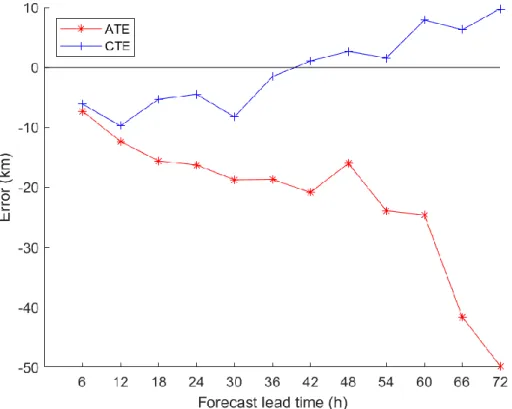
2006-2015 year. ... 16 Figure 3.5. Hourly mean along-track bias and cross-track bias of WRF run for all tropical cyclones in

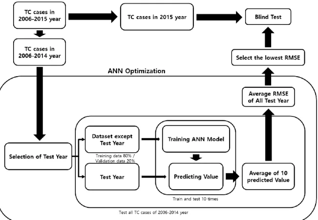
the 2006-2015 year. ... 17 Figure 3.6. ANN optimization (2006-2014) and blind testing (2015) process for TCs over the WNP.

... 18 Figure 3.7. Averaged RMSE of ANN optimization experiment for 24-hour forecast about (a) latitude

and (b) longitude for tropical cyclones in each 2006-2014 year. ... 19 Figure 3.8. Averaged RMSE of ANN optimization experiment for 48-hour forecast about (a) latitude

and (b) longitude for tropical cyclones in each 2006-2014 year. ... 20 Figure 3.9. Averaged RMSE of ANN optimization experiment for 72-hour forecast about (a) latitude

and (b) longitude for tropical cyclones in each 2006-2014 year. ... 21 Figure 3.10. Comparison of (a) latitude and (b) longitude of tropical cyclone after 24 hours between

ANN and best track. Comparison of (c) latitude and (d) longitude of tropical cyclone after 48 hours between ANN and best track. Comparison of (e) latitude and (f) longitude of tropical cyclone after 72 hours between ANN and best track. The black line indicates the identity line (y=x); the red line is the fitted line. ... 23

(10)

Figure 3.11. Output selection method for ANN results. Excluded ANN defined as EXANN. The blue (green; red) square is a range of ANN (WRF; EXANN) results. The range of green square is defined by MAEs of predicted latitude and longitude by WRF. OB is observation, and FC is the forecast position of WRF. ... 24 Figure 3.12. The number of excluded ANN for 24-hour forecast of (a) latitude and (b) longitude, for

48-hour forecast of (c) latitude and (d) longitude, and for 72-hour forecast of (e) latitude and (f) longitude with tropical cyclones in the 2015 year by output selection. ... 25 Figure 3.13. Comparison of (a) latitude and (b) longitude of tropical cyclone after 24 hours between

EXANN and best track. Comparison of (c) latitude and (d) longitude of tropical cyclone after 48 hours between EXANN and best track. Comparison of (e) latitude and (f) longitude of tropical cyclone after 72 hours between EXANN and best track. The black line indicates the identity line (y=x); the red line is the fitted line. ... 26 Figure 3.14. Track position error of ANN, EXANN, WRF for tropical cyclones for (a) 24-hour, (b) 48-

hour, and (c) 72-hour forecast in the 2015 year. ... 28 Figure 3.15. Track position error of EXANN, WRF for TCs in the 2015 year with descending order

about TPE of WRF for (a) 24-hour, (b) 48-hour, and (c) 72-hour forecast. ... 29 Figure 3.16. Track position error difference between EXANN and WRF for TCs in the 2015 year with

descending order about TPE of WRF for (a) 24-hour, (b) 48-hour, and (c) 72-hour forecast. The red line indicates the fitted line for EXANN-WRF with descending order about the TPE of WRF.

The blue line indicates the fitted line for ANN-WRF with descending order about the TPE of WRF.

... 30 Figure 3.17. Mean track position error of ANN, EXANN, WRF about (a) 24-hour, (b) 48-hour, and (c)

72-hour forecast for all TCs in the 2015 year. ... 31 Figure 3.18. Mean (a) along-track bias and (b) cross-track bias of ANN, EXANN, WRF averaged for

all tropical cyclones in the 2006-2015 year... 32 Figure 4.1. (a) Silhouette coefficient value plot for each number of clusters. (b) The number of negative

silhouette coefficient values included in each cluster from 2 to 10. ... 34

(11)

Figure 4.2. Four types of (a) TCs in the 2006-2015 year and (b) TCs in the 2015 year from k-means clustering result based on WRF simulations in the 2006-2015 year. Map for clustering result of.

Dodger blue is cluster 1, blue is cluster 2, green is cluster 3, orange is cluster 4, such as Figure 4.1.(a). ... 35 Figure 4.3. Mean track position error of ANN, EXANN, WRF averaged about (a) 24-hour, (b) 48-hour,

and (c) 72-hour forecast for TCs in each cluster about tropical cyclones of the 2015 year. ... 36

(12)

List of Tables

Table 2.1. Numerical weather model configuration. ... 4

Table 2.2. Forecast information and initial time of 106 TCs, which occurred from June to November in the 2006-2015 year over WNP. The interval of forecast initial time is 12 hours. ... 4

Table 2.3. Description of predictor used for training and testing ANN. ... 10

Table 4.1. Average of silhouette coefficient values for each number of cluster k from 2 to 10. ... 34

Table 5.1. ANN optimization for the number of neurons in each hidden layer... 37

(13)

Chapter Ⅰ Introduction

A tropical cyclone (TC) is a kind of natural disaster characterized by a low-pressure center, closed low-level atmospheric circulation, and a spiral arrangement of thunderstorms. TC can cause a considerable amount of social and economic damage with torrential rainfall, flash flood, and strong wind. East Asia and North America contribute to 88 % of financial loss by TC (Mendelsohn et al., 2012) and about 4 TCs occurred over the western North Pacific (WNP) have annually influenced Korea and Japan (Wu et al., 2004). There are typical cases that caused severe damage in Korea. Typhoon Rusa in 2002 broke recorded daily rainfall as 879.5 mm in Gangneung in the eastern coastal region of Korea, and high waves and astronomical high tide induced severe disaster in the coastal area while Typhoon Maemi (Typhoon 0314) passed (Kawai et al., 2005; Lee and Choi, 2010). TC can be assessed based on a model calculation to estimate losses of it (Rumpf et al., 2009; Lee et al., 2018). For mitigating and preparing significant damage and injury by TC, it is necessary to predict TC track accurately.

Atmospheric phenomena have been simulated and predicted with numerical and statistical models (Jin et al., 2016; Knaff et al., 2003; Neumann and Hope, 1972; Xu and Neumann, 1985). Despite advancements in observations and high computing system for the models, simulation still has a systematic error because of uncertainties in the computation of model and initial conditions. In order to reduce forecast error, there has been a lot of effort to improve forecast models related to physical processes, convection, ocean feedback and resolution (Islam et al., 2015; Park et al., 2008; Soden and Held, 2006; Kendon et al., 2012). Also, the performance of the forecast models has been improved by techniques related to initial condition (Kwon and Cheong, 2010; Cha et al., 2013), forcing data (Kang et al., 2005; Moon et al., 2019) and model output (Piani et al., 2010; Dosio and Paruolo, 2011).

Another method to predict atmospheric characteristics is machine learning (ML). ML is one kind of statistical models that capture non-linearities and complex relations from sample data based on scientific algorithms with computer systems. With the current emergence of machine learning technology as a new application field of supercomputing, many researchers have tried to predict TC track as well as weather and other natural disasters through the technique. Chaudhuri et al. (2015) used multilayer feed-forward neural nets with different architectures to forecast track and intensity of TCs over the North Indian Ocean with 6, 12, and 24 hours. Their high performed model was compared with other neural networks which have different architecture. Moradi et al. (2016) applied a sparse recurrent neural network for trajectory prediction of Atlantic hurricanes. They defined the center of hurricanes as two sequences and arranged two sequences on the sides of a grid, with one on the top and the other on the left-hand side. Zhang et al. (2018) handled spatial correlations in the data by matrix neural network without vectorization of cyclone trajectories. The neural network can adjust the input feature to any size,

(14)

such as 2D for each input unit. Rüttgers et al. (2019) predicted typhoon tracks using a generative adversarial network with a satellite image. They generated a future cloud image of TC by using cloud image satellite data for predicting the coordinate of a typhoon center. In the previous researches, machine learning was trained to identify the center of TC in a satellite image or to predict the trajectory of TC with meteorological data based on observation. The models were trained by input data about current or past TC without predicted future TC. The numerical weather model has been operated for predicting atmospheric phenomena, and it can produce predicted future atmospheric characteristics.

With numerical model data, machine learning can generate more accurate output for predicting atmospheric characteristics.

TC tracks in the WNP have different characteristics according to the location of track and environment.

By this feature, the numerical model generates the different performance of the TC track forecast depending on where it passes. Several studies tried to classify TC trajectories into a fixed number in order to find the characteristics of various TC tracks. Kim et al. (2011) used the fuzzy c-means clustering method to classify 855 TC tracks in the WNP during the 1965-2006 year. The cases were classified with 7 clusters, which have characteristics of landfall, track distance, and track shape. These clusters were analyzed by large-scale environments for the reason each track has the features. In addition, Kim et al.

(2016) classified TC tracks in WNP in the 1979-2013 year using a self-organizing map. The TC tracks were divided into 5 clusters, and TC genesis frequency was interpreted by intraseasonal and interannual features for each cluster. Zhang and Chan et al. (2013) tried to find mechanisms for elucidating TC track recurvature and landfall. In this process, the decision tree, which is one of data mining method for selecting features, was used for classifying. For the searching pattern of track forecast, it is necessary to analyze the feature of predicted TC tracks with classification. Clustering method is used in this study for finding features of ANN effect on TC tracks predicted by WRF.

In this study, we simulated TC cases for ten years (from 2006 to 2015) with Weather Research and Forecasting (WRF) model and trained artificial neural network (ANN) by TC information with predicted TC track by WRF. Methodology with WRF and ANN configuration are described in Chapter 2. Chapter 3 includes analyzing the performance of WRF model and optimizing ANN. Clustering analysis of model results in the 2015 year among ten years is presented in Chapter 4. The summary and discussion of this study are given in Chapter 5.

(15)

Chapter Ⅱ

Methodology and Dataset

2.1 Numerical Model Simulation

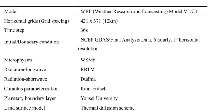
WRF model version 3.7.1 (Skamarock and Klemp, 2008), which is one kind of regional climate model, was used to generate six-hourly TC track data for three days. The horizontal resolution was 12 km, and the grid numbers of the domain were 421 x 371. Center of the model domain was defined as latitude which is more northward 10 ° than latitude of initial TC center and longitude which is less eastward 10°

than longitude of initial TC center when the TC center was under 20°N, and it was defined latitude which is more northward 10 ° than latitude of initial TC center and longitude of initial TC center when the TC center was over 20 °N. Vertical levels from the surface to the top of the atmosphere were 35, and the top of the atmosphere was 50 hPa in the domain. The model time step was 36 s. Model simulations were 72 hours of forecasts for TC cases over the WNP. NCEP final (FNL) Operational Global Analysis data with a 1 ° by 1 ° grid was used as the initial and boundary conditions for the WRF model. The model consisted of the WRF single-moment six-class microphysics scheme (Hong and Lim, 2006), Rapid Radiative Transfer Model long-wave radiation scheme (Mlawer et al., 1997), Dudhia short-wave radiation scheme (Dudhia, 1989), Kain-Fritsch cumulus parameterization scheme (Kain, 2004), Yonsei University planetary boundary layer scheme (Hong et al., 2006) and thermal diffusion scheme (Dudhia and Jimy, 1996). The model configuration was described in Table 2.1.

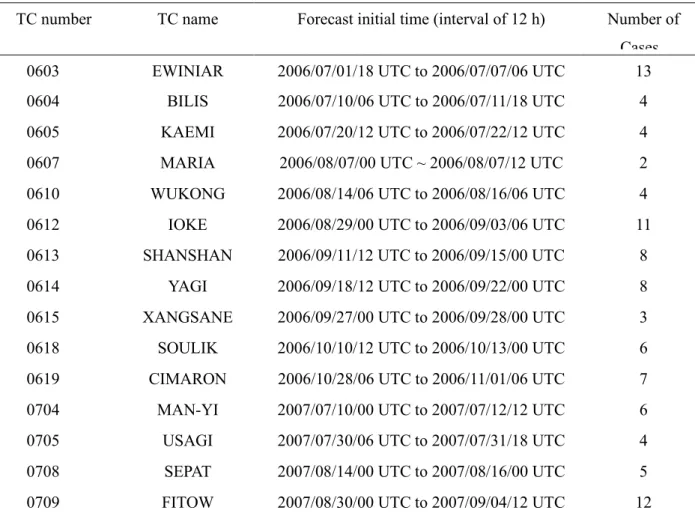
TCs over the WNP from June to November in the 2006-2015 year were simulated. TC can classify four categories about maximum wind speed with tropical depression (< 33 kts), tropical storm (34 - 47 kts), severe tropical storm (48 - 63 kts), and typhoon (> 64 kts). WRF model simulated the TCs of which intensity was over a tropical storm with interval of 12 hours. Totally 106 TCs were simulated, and WRF was run 666 times for each initial condition (Table 2.2). The 6-hourly location of TC center was defined by the minimum pressure in the sea level pressure field (Feser and von Storch, 2008a).

(16)

Table 2.1. Numerical weather model configuration.

Model WRF (Weather Research and Forecasting) Model V3.7.1

Horizontal grids (Grid spacing) 421 x 371 (12km)

Time step 36s

Initial/Boundary condition NCEP GDAS/Final Analysis Data, 6 hourly, 1° horizontal resolution

Microphysics WSM6

Radiation-longwave RRTM

Radiation-shortwave Dudhia

Cumulus parameterization Kain-Fritsch Planetary boundary layer Yonsei University

Land surface model Thermal diffusion scheme

Table 2.2. Forecast information and initial time of 106 TCs, which occurred from June to November in the 2006-2015 year over WNP. The interval of forecast initial time is 12 hours.

TC number TC name Forecast initial time (interval of 12 h) Number of Cases

0603 EWINIAR 2006/07/01/18 UTC to 2006/07/07/06 UTC 13

0604 BILIS 2006/07/10/06 UTC to 2006/07/11/18 UTC 4

0605 KAEMI 2006/07/20/12 UTC to 2006/07/22/12 UTC 4

0607 MARIA 2006/08/07/00 UTC ~ 2006/08/07/12 UTC 2

0610 WUKONG 2006/08/14/06 UTC to 2006/08/16/06 UTC 4

0612 IOKE 2006/08/29/00 UTC to 2006/09/03/06 UTC 11

0613 SHANSHAN 2006/09/11/12 UTC to 2006/09/15/00 UTC 8

0614 YAGI 2006/09/18/12 UTC to 2006/09/22/00 UTC 8

0615 XANGSANE 2006/09/27/00 UTC to 2006/09/28/00 UTC 3

0618 SOULIK 2006/10/10/12 UTC to 2006/10/13/00 UTC 6

0619 CIMARON 2006/10/28/06 UTC to 2006/11/01/06 UTC 7

0704 MAN-YI 2007/07/10/00 UTC to 2007/07/12/12 UTC 6

0705 USAGI 2007/07/30/06 UTC to 2007/07/31/18 UTC 4

0708 SEPAT 2007/08/14/00 UTC to 2007/08/16/00 UTC 5

0709 FITOW 2007/08/30/00 UTC to 2007/09/04/12 UTC 12

(17)

0710 DANAS 2007/09/08/06 UTC 1

0714 LEKIMA 2007/10/01/00 UTC 1

0715 KROSA 2007/10/03/06 UTC to 2007/10/04/18 UTC 4

0723 MITAG 2007/11/21/18 UTC to 2007/11/24/06 UTC 6

0724 HAGIBIS 2007/11/21/18 UTC to 2007/11/24/06 UTC 6

0806 FENGSHEN 2008/06/20/00 UTC to 2008/06/22/00 UTC 3

0808 FUNG-WONG 2008/07/26/06 UTC 1

0812 NURI 2008/08/19/06 UTC ~ 2008/08/19/18 UTC 2

0813 SINLAKU 2008/09/10/00 UTC to 2008/09/17/12 UTC 16

0814 HAGUPIT 2008/09/20/12 UTC to 2008/09/21/12 UTC 3

0815 JANGMI 2008/09/26/00 UTC to 2008/09/27/12 UTC 4

0908 MORAKOT 2009/08/04/18 UTC to 2009/08/07/06 UTC 6

0910 VAMCO 2009/08/18/18 UTC to 2009/08/22/18 UTC 9

0912 DUJUAN 2009/09/05/06 UTC to 2009/09/06/18 UTC 4

0914 CHOI-WAN 2009/09/14/00 UTC to 2009/09/17/00 UTC 7

0916 KETSANA 2009/09/27/00 UTC 1

0917 PARMA 2009/09/30/06 UTC to 2009/10/09/18 UTC 20

0918 MELOR 2009/10/01/06 UTC to 2009/10/05/06 UTC 9

0919 NEPARTAK 2009/10/10/06 UTC ~ 2009/10/10/18 UTC 2

0920 LUPIT 2009/10/16/12 UTC to 2009/10/23/12 UTC 15

0921 MIRINAE 2009/10/28/06 UTC to 2009/10/30/06 UTC 5

0922 NIDA 2009/11/25/00 UTC to 2009/11/27/12 UTC 6

1002 CONSON 2010/07/13/12 UTC to 2010/07/14/12 UTC 3

1004 DIANMU 2010/08/09/12 UTC 1

1006 LIONROCK 2010/08/29/18 UTC 1

1011 FANAPI 2010/09/16/18 UTC ~ 2010/09/17/06 UTC 2

1013 MEGI 2010/10/15/00 UTC to 2010/10/20/12 UTC 11

1014 CHABA 2010/10/25/18 UTC to 2010/10/27/06 UTC 4

1105 MEARI 2011/06/23/00 UTC ~ 2011/06/24/00 UTC 2

1106 MA-ON 2011/07/13/12 UTC to 2011/07/21/00 UTC 16

1108 NOCK-TEN 2011/07/27/00 UTC 1

1109 MUIFA 2011/07/29/06 UTC to 2011/08/05/18 UTC 16

1110 MERBOK 2011/08/04/18 UTC to 2011/08/06/06 UTC 4

(18)

1111 NANMADOL 2011/08/24/12 UTC to 2011/08/27/12 UTC 7

1112 TALAS 2011/08/26/00 UTC to 2011/09/01/12 UTC 14

1115 ROKE 2011/09/14/06 UTC to 2011/09/18/18 UTC 10

1116 SONCA 2011/09/16/12 UTC ~ 2011/09/17/00 UTC 2

1119 NALGAE 2011/09/28/18 UTC to 2011/09/30/18 UTC 5

1203 MAWAR 2012/06/02/18 UTC 1

1204 GUCHOL 2012/06/14/12 UTC to 2012/06/16/12 UTC 4

1209 SAOLA 2012/07/29/12 UTC to 2012/07/31/00 UTC 4

1210 DAMREY 2012/07/30/00 UTC ~ 2012/07/30/12 UTC 2

1211 HAIKUI 2012/08/04/12 UTC to 2012/08/06/00 UTC 4

1213 KAI-TAK 2012/08/14/00 UTC to 2012/08/15/00 UTC 3

1214 TEMBIN 2012/08/20/06 UTC to 2012/08/27/06 UTC 15

1215 BOLAVEN 2012/08/21/06 UTC to 2012/08/25/18 UTC 8

1216 SANBA 2012/09/12/00 UTC to 2012/09/14/12 UTC 6

1217 JELAWAT 2012/09/22/00 UTC to 2012/09/28/00 UTC 13

1218 EWINIAR 2012/09/25/12 UTC to 2012/09/26/12 UTC 3

1220 GAEMI 2012/10/02/12 UTC ~ 2012/10/03/00 UTC 2

1221 PRAPIROON 2012/10/08/12 UTC to 2012/10/16/00 UTC 16

1223 SON-TINH 2012/10/25/12 UTC to 2012/10/26/00 UTC 2

1224 BOPHA 2012/11/27/18 UTC 1

1307 SOULIK 2013/07/09/00 UTC to 2013/07/10/12 UTC 4

1311 UTOR 2013/08/10/18 UTC to 2013/08/12/06 UTC 3

1312 TRAMI 2013/08/19/00 UTC ~ 2013/08/19/12 UTC 2

1313 PEWA 2013/08/20/06 UTC to 2013/08/21/18 UTC 4

1319 USAGI 2013/09/18/00 UTC to 2013/09/20/00 UTC 5

1320 PABUK 2013/09/22/06 UTC to 2013/09/23/18 UTC 4

1323 FITOW 2013/10/01/18 UTC to 2013/10/03/18 UTC 5

1324 DANAS 2013/10/05/06 UTC ~ 2013/10/05/18 UTC 2

1325 NARI 2013/10/10/12 UTC to 2013/10/12/12 UTC 4

1326 WIPHA 2013/10/11/12 UTC to 2013/10/13/00 UTC 4

1327 FRANCISCO 2013/10/17/12 UTC to 2013/10/23/00 UTC 11

1328 LEKIMA 2013/10/21/18 UTC to 2013/10/23/06 UTC 3

1329 KROSA 2013/10/30/18 UTC to 2013/10/31/18 UTC 3

(19)

1330 HAIYAN 2013/11/05/06 UTC to 2013/11/07/18 UTC 6

1408 NEOGURI 2014/07/04/18 UTC to 2014/07/07/18 UTC 7

1409 RAMMASUN 2014/07/13/06 UTC to 2014/07/16/06 UTC 7

1410 MATMO 2014/07/18/12 UTC to 2014/07/22/00 UTC 8

1411 HALONG 2014/07/30/12 UTC to 2014/08/07/12 UTC 16

1413 GENEVIEVE 2014/08/09/00 UTC 1

1415 KALMAEGI 2014/09/13/18 UTC 1

1416 FUNG-WONG 2014/09/19/00 UTC to 2014/09/20/12 UTC 3

1417 KAMMURI 2014/09/25/12 UTC to 2014/09/27/00 UTC 4

1418 PHANFONE 201/09/30/06 UTC to 2014/10/03/06 UTC 7

1419 VONGFONG 2014/10/04/18 UTC to 2014/10/10/18 UTC 12

1420 NURI 2014/11/01/00 UTC to 2014/11/03/12 UTC 6

1509 CHAN-HOM 2015/07/01/12 UTC to 2015/07/09/12 17

1510 LINFA 2015/07/03/18 UTC,2015/07/05/18 UTC,

2015/07/06/06 UTC

3

1511 NANGKA 2015/07/04/18 UTC to 2015/07/14/06 UTC 19

1513 SOUDELOR 2015/08/02/06 UTC to 2015/08/06/18 UTC 10

1514 MOLAVE 2015/08/08/06 UTC to 2015/08/10/18 UTC 6

1515 GONI 2015/08/15/18 UTC to 2015/08/22/06 UTC 13

1516 ATSANI 2015/08/16/00 UTC to 2015/08/22/00 UTC 13

1517 KILO 2015/09/03/18 UTC to 2015/09/08/06 UTC 10

1520 KROVANH 2015/09/16/18 UTC to 2015/09/18/06 UTC 4

1521 DUJUAN 2015/09/24/00 UTC to 2015/09/26/00 UTC 5

1523 CHOI-WAN 2015/10/03/06 UTC, 2015/10/04/06 UTC 2

1524 KOPPU 2015/10/14/12 UTC to 2015/10/18/00 UTC 7

1525 CHAMPI 2015/10/15/00 UTC to 2015/10/22/00 UTC 14

Total 666

(20)

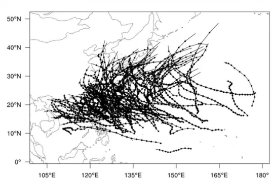
Figure 2.1. Best track of Regional Specialized Meteorological Centers Tokyo which is over Tropical cyclone from June to November in 2006-2015 for WRF simulation in this study.

2.2 Artificial Neural Network (ANN) Regression

ANN is based on an interconnected structure that is inspired by operations and connectivity of biological neurons in human brain (Özçelik et al., 2010; Tiryaki and Aydın, 2014, Yang et al., 2018). It is constructed with input layer, hidden layer, and output layer and feature neurons of each layer are interconnected with weight and bias. The neurons in ANN are trained for a target variable, and neural network is tuned by a back-propagation algorithm. It is basic type of neural net compared to convolutional neural network or recurrent neural network. In previous researches, ANN was used for regression problems because it has capability of finding pattern of non-linearities and complex relations.

In this study, ANN was built by the Keras open-source library. We adapted the rectified linear unit (ReLU) (Hahnloser et al., 2000) for the activation function and the adaptive moment estimation (ADAM) optimizer (Kingma and Ba, 2014) for the optimization function. ANN model in this study had two hidden layers, and sensitivity tests for the number of neurons in each hidden layer were conducted considering the performance of output. An epoch of the ANN was 500, and we applied to mean absolute error for loss function.

2.3 Datasets for Training ANN

The data employed in this study were separated as TC track, atmospheric dynamics, and numerical model output. TC track included a date, the coordinate of TC center, minimum sea-level pressure of

(21)

initial TC, and atmospheric dynamics included zonal wind (U), meridional wind (V). Numerical model output included the coordinates of predicted TC center after 6-72 hours.

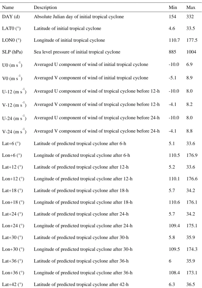
In TC track, historical data was included. The historical intensity and track for TC were extracted from the best track of Regional Specialized Meteorological Centers (RSMC) Tokyo. Best track data includes the date, locations, minimum sea level pressure (SLP), maximum wind speed (MWS), classification of TC during the life cycle of a TC with a 6-hour interval. Julian day, latitude and longitude were used as independent variables. DAY is a parameter for the date, which was calculated as the absolute value of the initial yearday called Julian day. In the case of the intensity of TC, SLP was used as an indicator of initial TC intensity even though both SLP and MWS represent the intensity of TC. In atmospheric dynamics, meteorological data was included. For the meteorological data, U and V were from European Centre for Medium-Range Weather Forecasts ERA-interim (ECMWF ERA-Interim) with a 6-hour interval and 0.70° by 0.70° horizontal resolution. We averaged U component and V component of wind from a square frame around the typhoon center of which length is 500 km. The averaging generates representative U and V of TC. U and V in initial time with U and V before 12 hours and 24 hours were used as input data together.

The numerical model output consists of predicted atmospheric characteristics. Sea level pressure was used for finding the center of TC in the model domain. The coordinates of TC center from 6 hours to 72 hours that are12 predictors were used as independent variables.

(22)

Table 2.3. Description of predictor used for training and testing ANN.

Name Description Min Max

DAY (d) Absolute Julian day of initial tropical cyclone 154 332

LAT0 (°) Latitude of initial tropical cyclone 4.6 33.5

LON0 (°) Longitude of initial tropical cyclone 110.7 177.5

SLP (hPa) Sea level pressure of initial tropical cyclone 885 1004 U0 (m s^-1) Averaged U component of wind of initial tropical cyclone -10.0 6.9 V0 (m s^-1) Averaged V component of wind of initial tropical cyclone -5.1 8.9 U-12 (m s^-1) Averaged U component of wind of tropical cyclone before 12-h -10.0 8.0 V-12 (m s^-1) Averaged V component of wind of tropical cyclone before 12-h -4.1 8.2 U-24 (m s^-1) Averaged U component of wind of tropical cyclone before 24-h -10.0 8.0 V-24 (m s^-1) Averaged V component of wind of tropical cyclone before 24-h -4.1 8.8 Lat+6 (°) Latitude of predicted tropical cyclone after 6-h 5.1 33.6 Lon+6 (°) Longitude of predicted tropical cyclone after 6-h 110.5 176.9 Lat+12 (°) Latitude of predicted tropical cyclone after 12-h 5.2 33.6 Lon+12 (°) Longitude of predicted tropical cyclone after 12-h 110.1 176.6 Lat+18 (°) Latitude of predicted tropical cyclone after 18-h 5.7 34.2 Lon+18 (°) Longitude of predicted tropical cyclone after 18-h 110.6 176.1 Lat+24 (°) Latitude of predicted tropical cyclone after 24-h 5.7 34.2 Lon+24 (°) Longitude of predicted tropical cyclone after 24-h 109.4 175.1 Lat+30 (°) Latitude of predicted tropical cyclone after 30-h 5.8 35.9 Lon+30 (°) Longitude of predicted tropical cyclone after 30-h 109.5 174.3 Lat+36 (°) Latitude of predicted tropical cyclone after 36-h 6 35.9 Lon+36 (°) Longitude of predicted tropical cyclone after 36-h 108.4 173.1 Lat+42 (°) Latitude of predicted tropical cyclone after 42-h 6.3 36.5

(23)

Lon+42 (°) Longitude of predicted tropical cyclone after 42-h 107.2 172.1 Lat+48 (°) Latitude of predicted tropical cyclone after 48-h 6.4 38.2 Lon+48 (°) Longitude of predicted tropical cyclone after 48-h 106.3 171 Lat+54 (°) Latitude of predicted tropical cyclone after 54-h 6.5 41 Lon+54 (°) Longitude of predicted tropical cyclone after 54-h 105.4 169.8 Lat+60 (°) Latitude of predicted tropical cyclone after 60-h 6.5 44.4 Lon+60 (°) Longitude of predicted tropical cyclone after 60-h 104.3 168.8 Lat+66 (°) Latitude of predicted tropical cyclone after 66-h 6.7 47.2 Lon+66 (°) Longitude of predicted tropical cyclone after 66-h 102.9 167.9 Lat+72 (°) Latitude of predicted tropical cyclone after 72-h 6.8 50.4 Lon+72 (°) Longitude of predicted tropical cyclone after 72-h 100.8 167.5

(24)

Chapter Ⅲ

WRF Simulation and ANN Optimization

3.1 Performance of TC Forecast using WRF

In order to assess the performance of the models, it is necessary to select evaluation criteria. In this study, mean bias error (MBE), mean absolute error (MAE), root mean square error (RMSE), and coefficient of determination (R²) were chosen to evaluate the output of the models. The MBE indicates better performance when its value is close to zero. The MAE and RMSE represent better performance when their value is lower. The R² is used to analyze how one variable can be explained by the other variable. The other variable can explain well if the value of the R² is close to 1. The MBE, MAE, RMSE, and R²are defined as followed formulas:

MBE = 1

𝑁∑(𝐹_𝑖− 𝑂_𝑖)

𝑁

𝑖=1

(1)

MAE = 1

𝑁∑|(𝐹_𝑖− 𝑂_𝑖)|

𝑁

𝑖=1

(2)

RMSE = √1

𝑁∑(𝐹_𝑖− 𝑂_𝑖)²

𝑁

𝑖=1

(3)

𝑅²= 1 −𝑆𝑆_{𝑅𝑒𝑔𝑟𝑒𝑠𝑠𝑖𝑜𝑛}

𝑆𝑆_{𝑇𝑜𝑡𝑎𝑙} (4)

where N is the number of cases, 𝐹_𝑖 is predicted values, 𝑂_𝑖 is observed values, 𝑆𝑆_{𝑅𝑒𝑔𝑟𝑒𝑠𝑠𝑖𝑜𝑛} is sum squared regression error, and 𝑆𝑆_{𝑇𝑜𝑡𝑎𝑙} is sum squared total error.

The tracking error referred to as track position error (TPE) is the great-circle distance between TC forecast position and the best track position. Distance between forecast (𝜑_𝑠, 𝜆_𝑠) and best track (𝜑₀, 𝜆₀) latitude and longitude of TC on spherical earth can be calculated from the haversine formula (Neumann and Pelissier, 1981; Powell & Aberson, 2001; Moon et al., 2018):

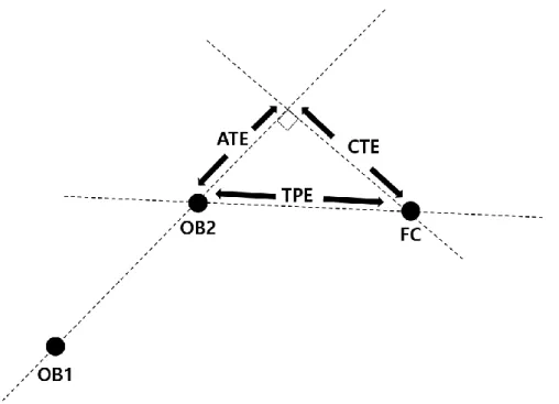
𝑇𝑃𝐸 = 111.11𝑐𝑜𝑠⁻¹[𝑠𝑖𝑛𝜑₀𝑠𝑖𝑛𝜑_𝑠+ 𝑐𝑜𝑠𝜑₀𝑐𝑜𝑠𝜑_𝑠𝑐𝑜𝑠(𝜆₀− 𝜆_𝑠)] (5) The TPE is the criterion about the quality of track error, but it doesn't contain information about the difference in speed and direction between forecast and best track of TC. The TPE can be divided into two components to be explained about speed and direction as an along-track error (ATE) and cross- track error (CTE). The ATE occurred when predicted TC move faster or slower than observed TC

(25)

according to the direction of observation. The ATE can be defined as that formula:

ATE =(𝑂𝐵1 𝑂𝐵2⃗⃗⃗⃗⃗⃗⃗⃗⃗⃗⃗⃗⃗⃗⃗⃗⃗⃗⃗ ∙ 𝑂𝐵1 𝐹𝐶⃗⃗⃗⃗⃗⃗⃗⃗⃗⃗⃗⃗⃗⃗⃗⃗ )

‖𝑂𝐵1 𝑂𝐵2⃗⃗⃗⃗⃗⃗⃗⃗⃗⃗⃗⃗⃗⃗⃗⃗⃗⃗⃗ ‖ − ‖𝑂𝐵1 𝑂𝐵2⃗⃗⃗⃗⃗⃗⃗⃗⃗⃗⃗⃗⃗⃗⃗⃗⃗⃗⃗ ‖ (6) The ATE has a positive value if predicted TC moves faster than observed TC and has negative value if predicted TC moves slower than observed TC. The CTE determines how much predicted TC moves toward the side of observed TC direction. The CTE can be defined as that formula:

CTE = √‖𝑂𝐵1 𝐹𝐶⃗⃗⃗⃗⃗⃗⃗⃗⃗⃗⃗⃗⃗⃗⃗⃗ ‖²−(𝑂𝐵1 𝑂𝐵2⃗⃗⃗⃗⃗⃗⃗⃗⃗⃗⃗⃗⃗⃗⃗⃗⃗⃗⃗ ∙ 𝑂𝐵1 𝐹𝐶⃗⃗⃗⃗⃗⃗⃗⃗⃗⃗⃗⃗⃗⃗⃗⃗ )²

‖𝑂𝐵1 𝑂𝐵2⃗⃗⃗⃗⃗⃗⃗⃗⃗⃗⃗⃗⃗⃗⃗⃗⃗⃗⃗ ‖² (7) The CTE has a positive value if predicted TC moves the right side of observed TC direction and has negative value if predicted TC moves left side of observed TC direction in the Northern hemisphere (Aemisegger, 2009).

Figure 3.1. Criteria for estimating forecast errors based on length, speed and direction. OB1 is the observation at time t, OB2 is the observation at time t+1, FC is the forecast at time t+1.

(26)

Simulated TC cases in the 2006-2015 year were compared with the best track of RSMC. Predicted latitude and longitude of WRF were compared with latitude and longitude of best track data separately.

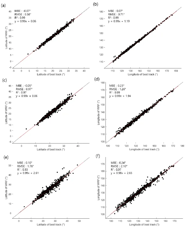
The MBEs of predicted latitude after 24, 48, and 72 hours were -0.07 °, -0.05 °, and 0.10 °. The RMSEs of predicted latitude after 24, 48, and 72 hours were 0.58 °, 0.97 °, and 1.76 °. WRF tends to simulate TCs more southward than best track, but TCs predicted by WRF move more northward when forecast lead time passes. The MBEs of predicted longitude after 24, 48, and 72 hours were 0.07 °, 0.23 °, and 0.24 °. The RMSEs of predicted longitude after 24, 48, and 72 hours were 0.71 °, 1.26 °, and 2.10 °.

WRF tends to simulate TCs more eastward in all forecast lead time. Forecast error of WRF is an effect on longitude than latitude, and the RMSEs of latitude and longitude are increasing when forecast lead time passes (Figure 3.2).

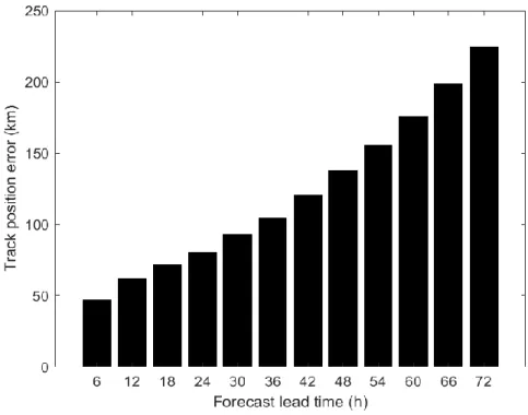
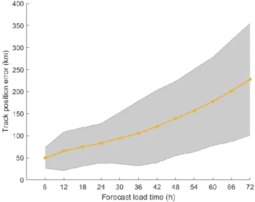
The average of the TPEs in all years described the general performance of predicting TC position in each forecast hour. Each TPEs of 6 hourly forecasts of TC position from 6 hours to 72 hours was 46.8, 62.1, 71.9, 80.4, 93.2, 104.4, 120.4, 137.7, 155.5, 175.4, 199.0, and 224.4 km (Figure 3.3). According to analyzing the TPE of TC forecast in each year separately, it represents that the numerical model generates the different performance of TC track forecast from 57.8 to 127 km after 24 hours, from 106.8 to 223.3 km after 48 hours, and from 172.4 to 355.1 km after 72 hours (Figure 3.4).

(27)

Figure 3.2. Comparison of (a) latitude and (b) longitude of tropical cyclone after 24 hours between WRF and best track. Comparison of (c) latitude and (d) longitude of tropical cyclone after 48 hours between WRF and best track. Comparison of (e) latitude and (f) longitude of tropical cyclone after 72

hours between WRF and best track. The black line indicates the identity line (y=x); the red line is the fitted line.

(28)

Figure 3.3. Hourly mean track position error of WRF run for all tropical cyclones in the 2006-2015 year.

Figure 3.4. Hourly mean track position error of WRF run for tropical cyclones with error spread in the 2006-2015 year.

(29)

Figure 3.5 describes the average of the ATE and CTE about the six-hourly TC position forecast. The ATE was decreasing when WRF had been simulated for more forecast lead time. WRF predicted TC position at a slower speed than observed TC position. The more WRF simulated about next time step of TC position, the slower predicted TC position was based on the direction of the observed TC position.

The CTE started with a negative value, but it had a positive value as of 42 hours. At the beginning of WRF simulation, the predicted TC position moved toward the left side of the observed TC position.

But, the predicted TC position gradually moved with the same direction of observed TC position and moved toward the right side of the observed TC position after 42 hours.

Figure 3.5. Hourly mean along-track bias and cross-track bias of WRF run for all tropical cyclones in the 2006-2015 year.

3.2 Optimization of Neurons in the Hidden Layer of ANN

ANN consists of three different kinds of the layer. The input and output layer are basic components to obtain input data and generate output from ANN. The number of neurons in the input layer is defined by the characteristic of input data, and the number of neurons in the output layer is specified by the problem, which should be solved with ANN. So, settings of input and output layer can be determined without difficulty. On the other hand, there is no theoretical determination of how many hidden layers and neurons make the best performance of ANN for each problem. For ANN optimization, it is

(30)

necessary to find the number of hidden layers and the number of neurons in each hidden layer (Carvalho et al., 2011; Mohammadhassani et al., 2013). The number of hidden layers is fixed as two, and the experiments of ANN optimization were set for testing the number of neurons in each hidden layer from 10 to 30 at two intervals. Totally different 121 architectures of ANN were tested in ANN optimization.

For producing a representative value of one ANN architecture, we set a process explained in Figure 3.6.

TCs of one year were used for test datasets, and rest data was divided into two parts as 80 % for calibration and 20 % for validation. Since ANN doesn't produce the same output whenever ANN is trained, we trained ANN 10 times and generated ten predicted values. All predicted values were averaged for extracting representative results about TCs of one year. Each representative result was extracted by testing TCs of each year in one experiment of ANN optimization. Lastly, averaged RMSE of each representative result was used for selecting the number of neurons that has the best performance.

The dataset of TCs in 2006 – 2014 years was used to do ANN optimization and TCs in the 2015 year was used for blinding test. We built two types of ANN models for predicting latitude and longitude separately.

Figure 3.6. ANN optimization (2006-2014) and blind testing (2015) process for TCs over the WNP.

(31)

Figure 3.7a represents the result of ANN optimization about the latitude forecast model for 24-hour forecast. The lowest RMSE of this optimization was 0.56 ° compared with 0.61 °, which is the RMSE of WRF latitude. The number of neurons that has the lowest RMSE is 26 and 10 neurons of each two hidden layers in order. Figure 3.7b represents the result of ANN optimization about longitude forecast model for 24-hour forecast. The lowest RMSE of this optimization was 0.66 ° which is lower than 0.72 ° that is the RMSE of WRF longitude. The number of neurons that has the lowest RMSE is 22 and 10 neurons of each two hidden layers in order. As a result, optimized ANN model for latitude had 26 and 10 neurons of each hidden layer and optimized ANN model for longitude had 22 and 10 neurons of each hidden layer sequentially.

Figure 3.7. Averaged RMSE of ANN optimization experiment for 24-hour forecast about (a) latitude and (b) longitude for tropical cyclones in each 2006-2014 year.

(32)

The result of ANN optimization about the latitude forecast model for 48-hour forecast is described in Figure 3.8a. The lowest RMSE of this optimization was 0.95 ° which is lower than 1.02 ° the RMSE of WRF latitude. The number of neurons that has the lowest RMSE is 18 and 14 neurons of each two hidden layers in order. The result of ANN optimization about longitude forecast model for 48-hour forecast is described in Figure 3.8b. The lowest RMSE of this optimization was 1.23 ° which is lower than 1.31 ° the RMSE of WRF longitude. The number of neurons that has the lowest RMSE is 10 and 12 neurons of each two hidden layers in order. Lastly, optimized ANN model for latitude had 18 and 14 neurons of each hidden layer and optimized ANN model for longitude had 10 and 12 neurons of each hidden layer sequentially.

(33)

Figure 3.9a represents the result of ANN optimization about the latitude forecast model for the 72- hour forecast. All results had lower RMSE than the RMSE of latitude from WRF. The lowest RMSE of this optimization was 1.67 ° compared with 1.83 °, which is the RMSE of WRF latitude. The number of neurons that has the lowest RMSE is 14 and 16 neurons of each two hidden layers in order. Figure 3.9b represents the result of ANN optimization about the longitude forecast model for the 72-hour forecast. RMSEs of this result were over the RMSE of longitude from WRF. The lowest RMSE of this optimization was 2.19 °, which is higher than 2.18 ° that is the RMSE of WRF longitude. The number of neurons that has the lowest RMSE is 18 and 10 neurons of each two hidden layers in order. As a result, the optimized ANN model for latitude had 14 and 16 neurons of each hidden layer, and the optimized ANN model for longitude had 18 and 10 neurons of each hidden layer sequentially.

(34)

Optimized ANN models for latitude and longitude were used for blind test about TCs in the 2015 year. The number of samples about TCs in 2015 years is 123 cases. The optimized ANN models were trained using TC cases in the 2006-2014 year and tested by TC cases in the 2015 year. In case of predicting latitude, MBEs for 24-hour, 48-hour, and 72-hour were 0.17 °, 0.36 °, and 0.28 ° and RMSEs for 24-hour, 48-hour, and 72-hour were 0.54 °, 0.86 °, and 1.44 °. ANN doesn’t have better performance than WRF except 72-hour for latitude forecast, and it predicted TC more northward than WRF. For predicting longitude, MBEs for 24-hour, 48-hour, and 72-hour were -0.15 °, -0.28 ° and -0.15 ° and RMSEs for 24-hour, 48-hour, and 72-hour were 0.64 °, 0.94 °, and 1.43 °. ANN also doesn't have better performance than WRF except 72-hour for longitude forecast. ANN predicted the longitude of TC more westward based on observation. Forecast results for 24-hour and 48-hour followed the trend of observation well despite the fact that those optimized ANN model predicted TC position worse than WRF. Through ANN was optimized by TC cases in 2006-2014 years, MBE, RMSE, and R² for 72-hour forecast represented that the result of ANN was better than WRF.

(35)

Figure 3.10. Comparison of (a) latitude and (b) longitude of tropical cyclone after 24 hours between ANN and best track. Comparison of (c) latitude and (d) longitude of tropical cyclone after 48 hours between ANN and best track. Comparison of (e) latitude and (f) longitude of tropical cyclone after 72

hours between ANN and best track. The black line indicates the identity line (y=x); the red line is the fitted line.

(36)

3.3 Post-Processing for ANN Output

Representative result of ANN was calculated by averaging outputs from ten times train and test because ANN generates different outputs at each time. There were some outputs which didn't have better performance. Output selection is needed to exclude unreasonable output, which can have a bad influence on ANN result. The range of output selection was set using MAE of latitude and longitude of WRF from the center of typhoon at forecast lead time. The range for output selection of latitude was calculated by averaging MAE of the predicted latitude of WRF, and range for output selection of longitude was calculated by averaging MAE of predicted longitude of WRF about all TCs in the 2006- 2015 year. Averaged MAEs of latitude forecast after 24-hour, 48-hour, and 72-hour were 0.44 km, 0.72 km, and 1.21 km. Averaged MAEs of longitude forecast after 24-hour, 48-hour, and 72-hour were 0.50 km, 0.94 km, and 1.53 km. Averaged ANN outputs which were in the range of output selection was used as excluded ANN (EXANN) results. If 10 ANN results are excluded, the last result is changed to the predicted position of WRF. Figure 3.12 describes the number of excluded ANN latitude and longitude for each tropical cyclone separately in the 2015 year. Averages of excluding cases in latitude for 24-hour, 48-hour, and 72-hour forecast were 3.24, 2.71, and 2.43. Averages of excluding cases in latitude for 24-hour, 48-hour, and 72-hour forecast were 2.80, 2.53, and 2.50.

Figure 3.11. Output selection method for ANN results. Excluded ANN defined as EXANN. The blue (green; red) square is a range of ANN (WRF; EXANN) results. The range of green square is defined

by MAEs of predicted latitude and longitude by WRF. OB is observation, and FC is the forecast position of WRF.

(37)

Figure 3.12. The number of excluded ANN for 24-hour forecast of (a) latitude and (b) longitude, for 48-hour forecast of (c) latitude and (d) longitude, and for 72-hour forecast of (e) latitude and (f)

longitude with tropical cyclones in the 2015 year by output selection.

(38)

Figure 3.13. Comparison of (a) latitude and (b) longitude of tropical cyclone after 24 hours between EXANN and best track. Comparison of (c) latitude and (d) longitude of tropical cyclone after 48

hours between EXANN and best track. Comparison of (e) latitude and (f) longitude of tropical cyclone after 72 hours between EXANN and best track. The black line indicates the identity line

(y=x); the red line is the fitted line.

(39)

In Figure 3.13, MBEs of EXANN about latitude for 24-hour, 48-hour, and 72-hour were 0.12 °, 0.20 °, and 0.24 ° and RMSEs of them were 0.42 °, 0.72 °, and 1.27 °. The output selection decreases the tendency of ANN to predict TC position more northward. Also, output selection generated the result which had a lower error than ANN. In Figure 3.13, MBEs of EXANN about longitude for 24-hour, 48- hour, and 72-hour were 0.03 °, -0.04 °, and 0.06 ° and RMSEs of them were 0.46 °, 0.76 °, and 1.43 °.

Predicted TC positions of ANN, which moved more westward than observation, were excluded by output selection. Although EXANN had a similar error with ANN for 72-hour forecast, EXANN has better performance than ANN for 24-hour and 48-hour forecast.

Figure 3.14 represents TPE of predicted TC position from ANN and EXANN for TCs in 2015 year.

The performances of ANN and EXANN were different in each case. The number of cases that were improved by output selection was 68 cases for 24-hour forecast, 66 cases for 48-hour forecast, and 63 cases for 72-hour forecast among 123 cases. Mean improvements for 24-hour, 48-hour, and 72-hour forecast were 35.1 %, 30.4 %, and 26.2 %. ANN could be improved by excluding outlier output of ANN using output selection in this study. Figure 3.15 describes TPE of WRF with descending order of it with TPE of EXANN. Higher TPE of EXANN appeared at lower TPE of WRF. The output selection improved the performance of predicting TC position more when WRF gets high TPE of TC forecast track. Also, Figure 3.16 describes how ANN and EXANN affect TPE of WRF with difference of EXANN and WRF for descending order of WRF. For 24-hour and 48-hour forecast, ANN and EXANN had similar improvement compared with TPE of WRF when TPE of WRF was larger. However, ANN can improve the performance of WRF more than EXANN when TPE of WRF was larger for 72-hour forecast. EXANN had lower TPE than TPE of ANN when TPE of WRF was lower.

TPE of ANN was larger than TPE of WRF for 24-hour and 48-hour forecast. TPE of EXANN was lower than TPE of WRF for all forecast lead time. For 72-hour forecast, the TPE of ANN was 164.4 km that is lower than the TPE of WRF, which is 182.5 km. Output selection improved the performance of ANN, and these forecast models using ANN and output selection improved the performance of WRF.

The ANN model for 72-hour forecast had greater improvement among three different models with 10.0 % for 24-hour, 13.0 % for 48-hour, and 15.5 % for 72-hour. Through analyzing the ANN model for 72- hour forecast, which had the best improvement, both ANN and EXANN have lower absolute ATE and CTE than WRF in Figure 3.18. ANN has an impact on WRF by correcting the speed and direction of WRF. For the correcting speed of WRF according to the direction of observation, ANN reduced more ATE than EXANN, but EXANN had better performance than ANN for correcting the direction of WRF according to the direction of observation.

(40)

Figure 3.14. Track position error of ANN, EXANN, WRF for tropical cyclones for (a) 24-hour, (b) 48-hour, and (c) 72-hour forecast in the 2015 year.

(41)

Figure 3.15. Track position error of EXANN, WRF for TCs in the 2015 year with descending order about TPE of WRF for (a) 24-hour, (b) 48-hour, and (c) 72-hour forecast.

(42)

Figure 3.16. Track position error difference between EXANN and WRF for TCs in the 2015 year with descending order about TPE of WRF for (a) 24-hour, (b) 48-hour, and (c) 72-hour forecast. The red line indicates the fitted line for EXANN-WRF with descending order about the TPE of WRF. The

blue line indicates the fitted line for ANN-WRF with descending order about the TPE of WRF.

(43)

Figure 3.17. Mean track position error of ANN, EXANN, WRF about (a) 24-hour, (b) 48-hour, and (c) 72-hour forecast for all TCs in the 2015 year.

(44)

Figure 3.18. Mean (a) along-track bias and (b) cross-track bias of ANN, EXANN, WRF averaged for all tropical cyclones in the 2006-2015 year.

(45)

Chapter Ⅳ

Analysis of Predicted TCs by ANN in 2015

4.1 K-Means Clustering and Silhouette Coefficient Value

Clustering is a method to group a set of objects which are more similar to each other than other sets of objects. It is used to identify characteristics of given data for understanding its pattern. The characteristics identified with clustering are more representative than the viewing value of data. In this study, k-means clustering, which is one of the popular clustering methods, was used for clustering analysis of ANN result. The k-means clustering distributes overall data in each group in which each observation closes with the mean of cluster. The AS-136 algorithm (Hartigan and Wong, 1979) was used for k-means clustering in this study. The predicted TC track by WRF was classified by the clustering algorithm.

The k parameter is the number of clustering group, and it should be defined before running k-means clustering. Defining the optimal number of clusters k was necessary to k-means clustering. Silhouette value is one of the useful methods to interpret and verify clusters with data. The silhouette coefficient is a measure of how well the clusters are divided and is a useful tool to assess the quality of the clustering result. The silhouette coefficient (s) represents the similarity of objects in its own cluster compared with other clusters, and it can be defined as,

𝑠(i) = 𝑏(𝑖) − 𝑎(𝑖) 𝑚𝑎𝑥{𝑎(𝑖), 𝑏(𝑖)}

where 𝑎(𝑖) is the mean of distances from 𝑖 to other data points in the same cluster and 𝑏(𝑖) is the mean of distances from 𝑖 to all data points in any other cluster which doesn’t include 𝑖. The silhouette range is from -1 to +1, and high silhouette value indicates that the object is similar to its own cluster and is not similar to other neighboring clusters.

4.2 Cluster Analysis of TC Track Forecast

The average of silhouette coefficient values is the highest when the number of clusters k is 2. But negative silhouette coefficient values, which indicate poorly fitting to the cluster, were considered for assessing the quality of the cluster. The number of clusters k was decided as four because it contains the lowest number of negative silhouette coefficient values in the number of k from 2 to 10, and it has the third-highest average of silhouette coefficient values.

(46)

Table 4.1. Average of silhouette coefficient values for each number of cluster k from 2 to 10.

Number of clusters k k=2 k=3 k=4 k=5 k=6 k=7 k=8 k=9 k=10 Average of silhouette

coefficient values 0.466 0.335 0.314 0.315 0.286 0.308 0.294 0.276 0.259

Figure 4.1. (a) Silhouette coefficient value plot for each number of clusters. (b) The number of negative silhouette coefficient values included in each cluster from 2 to 10.

Predicted 123 TCs by WRF in the 2015 year was analyzed from clustering result of WRF simulation in the 2006-2015 year (Figure 4.2). Cluster 1 includes 24 (19%) predicted cases in almost west of Japan.

Cluster 2 comprises 26 (21%) predicted cases that can affect Korea, Japan and China. Cluster 3 includes 17 (14%) predicted cases that are in south of China and can only affect China and eastern South Asia.

Cluster 4 comprises 56 (46%) predicted cases that are in west and south of Japan and can affect Japan.

The predicted TC positions by ANN had different performances in each cluster. For analyzing prediction of 24-hour and 48-hour forecast, ANN couldn’t predict TC position well in cluster 1. Output selection reduced error of ANN in all clusters and EXANN had better performance than WRF especially in cluster 1 and cluster 3. For analyzing result of 72-hour forecast, WRF of cluster 1 and cluster 2 couldn’t be improved with ANN, and output selection made ANN more useful output which was lower than WRF.

In cluster 3 and cluster 4, TPE of ANN and EXANN was lower than TPE of WRF, but output selection didn’t increase the performance of ANN more accurately (Figure 4.3).

(47)

Figure 4.2. Four types of (a) TCs in the 2006-2015 year and (b) TCs in the 2015 year from k-means clustering result based on WRF simulations in the 2006-2015 year. Map for clustering result of.

Dodger blue is cluster 1, blue is cluster 2, green is cluster 3, orange is cluster 4, such as Figure 4.1.(a).

(48)

Figure 4.3. Mean track position error of ANN, EXANN, WRF averaged about (a) 24-hour, (b) 48- hour, and (c) 72-hour forecast for TCs in each cluster about tropical cyclones of the 2015 year.

(49)

Chapter Ⅴ

Summary and Discussion

In this study, we simulated 106 TCs with 666 initial times from June to November in the 2006-2015 year over the WNP using WRF and corrected predicted position of TC with ANN. WRF output, TC track, and atmosphere dynamics were used as variables for training ANN. We targeted predicted TC positions after 24 hours, 48 hours, and 72 hours. WRF had an error of predicted track about TCs such as 80.4 km after 24 hours, 137.7 km after 48 hours, and 224.4 km after 72 hours. Before setting forecast models for the TC position based on ANN, we evaluated the performance of latitude and longitude prediction from WRF separately. WRF simulated TCs more southward than real track except for 72- hour forecast and simulated TCs more eastward than real track. Predicted TCs by WRF moved on the left side of the direction of observation early, and it was changed to a tendency to move on the right side of the direction of observation. Also, it moved slower than observation, and it caused improving the error of TC track prediction.

We set ANN models for latitude and longitude individually and test the sensitivity of the number of neurons in hidden layers. TCs in the 2006-2014 year were used for ANN optimization. ANN was trained and tested ten times, and all results were averaged. This process was done for each year, and results from each year were averaged for extracting representative value about types of ANN architecture. ANN models of latitude and longitude for each forecast lead time were optimized by the process (Table 5.1).

When TCs in the 2015 year were used for blind test about optimized ANN, ANN models predicted TC position more northward and westward than WRF. For reducing the outlier of the result of ANN, we define output selection based on the MAE of WRF. The result by output selection was defined as EXANN, and output selection reduced the error of ANN for each forecast lead time. EXANN had greater improvement when WRF had a higher error. EXANN could improve the performance of WRF prediction from 10% to 15.5% and change to a tendency to move close in the direction of observation.

Table 5.1. ANN optimization for the number of neurons in each hidden layer.

Forecast lead time 24-hour 48-hour 72-hour

Target Latitude Longitude Latitude Longitude Latitude Longitude

Number of neurons

Hidden

layer 1 26 22 18 10 14 18

Hidden

layer 2 10 10 14 12 16 10

(50)

The performance of WRF was different depending on where TCs were located. To do clustering analysis, TCs in this study were classified as four types of clusters based on k-means clustering according to the silhouette coefficient value. TCs were divided in the location of TCs such as western Pacific for cluster 1, south of Korea for cluster 2, Southeast Asia and China for cluster 3, and south of Japan for cluster 4. For 24-hour and 48-hour forecast, output selection removed outlier of ANN, which predicted TC position worse. EXANN improved the performance of WRF in cluster 1 and cluster 3 more than other clusters. For 72-hour forecast, ANN had lower error than EXANN in cluster 3 and cluster 4 even though EXANN was better than ANN in cluster 1 and cluster 2.

According to the results of this study, the accuracy of the predicted TC position by WRF can be improved by ANN. Output selection can eliminate worse result of ANN and make their quality better which had lower error than WRF. WRF can be improved not only with its schemes and external techniques but also with current technology of other fields such as machine learning. Technology that can explain complex relationships better than previous methods in the field of machine learning continues to be developed, and applying them to numerical models will generate higher improvement results. It is worthy of the application of other machine learning methods to predict more accurate position of TC.

ANN with TCs in the 2006-2015 year can be compared with WRF, but the number of samples in this study is less compared to previous research of applying machine learning. It is better to simulate more tropical cyclone cases to progress generalization of ANN. Also, Previous researchers used some variables such as satellite image, temperature and wind field, and their model which used those variables generated different results from result of this study. Not only variables in this study but also other variables like thermodynamic and variables of other pressure levels need to be tested how those variables affect the forecast of TC track.

(51)

Chpater Ⅵ References

Aemisegger, F. (2009). Tropical Cyclone Forecast Verification. ETH, 99pp.

Carvalho, A. R., Ramos, F. M., & Chaves, A. A. (2011). Metaheuristics for the feedforward artificial neural network (ANN) architecture optimization problem. Neural Computing and Applications, 20(8), 1273-1284.

Cha, D. H., & Wang, Y. (2013). A dynamical initialization scheme for real-time forecasts of tropical cyclones using the WRF model. Monthly Weather Review, 141(3), 964-986.

Chaudhuri, S., Dutta, D., Goswami, S., & Middey, A. (2015). Track and intensity forecast of tropical cyclones over the North Indian Ocean with multilayer feed forward neural nets. Meteorological Applications, 22(3), 563-575.

Dosio, A., & Paruolo, P. (2011). Bias correction of the ENSEMBLES high‐resolution climate change projections for use by impact models: Evaluation on the present climate. Journal of Geophysical Research: Atmospheres, 116(D16).

Dudhia, J., 1989: Numerical study of convection observed during the Winter Monsoon Experiment using a mesoscale two–dimensional model. J. Atmos. Sci., 46, 3077–3107.

Dudhia, Jimy, 1996: A multi-layer soil temperature model for MM5. the Sixth PSU/NCAR Mesoscale Model Users' Workshop.

Feser, F., & von Storch, H. (2008). A dynamical downscaling case study for typhoons in Southeast Asia using a regional climate model. Monthly Weather Review, 136(5), 1806-1815.

Hahnloser, R. H., Sarpeshkar, R., Mahowald, M. A., Douglas, R. J., & Seung, H. S. (2000). Digital selection and analogue amplification coexist in a cortex-inspired silicon circuit. Nature, 405(6789), 947.

Hartigan, J. A., & Wong, M. A. (1979). Algorithm AS 136: A k-means clustering algorithm. Journal of the Royal Statistical Society. Series C (Applied Statistics), 28(1), 100-108.

Hong, S.–Y., and J.–O. J. Lim, 2006: The WRF single–moment 6–class microphysics scheme (WSM6). J. Korean Meteor. Soc., 42, 129–151.

Hong, Song–You, Yign Noh, Jimy Dudhia, 2006: A new vertical diffusion package with an explicit treatment of entrainment processes. Mon. Wea. Rev., 134, 2318–2341.

(52)

Islam, T., Srivastava, P. K., Rico-Ramirez, M. A., Dai, Q., Gupta, M., & Singh, S. K. (2015). Tracking a tropical cyclone through WRF–ARW simulation and sensitivity of model physics. Natural Hazards, 76(3), 1473-1495.

Jin, C. S., Cha, D. H., Lee, D. K., Suh, M. S., Hong, S. Y., Kang, H. S., & Ho, C. H. (2016). Evaluation of climatological tropical cyclone activity over the western North Pacific in the CORDEX-East Asia multi-RCM simulations. Climate dynamics, 47(3-4), 765-778.

Kain, John S., 2004: The Kain–Fritsch convective parameterization: An update. J. Appl. Meteor., 43, 170–181.

Kang, H. S., Cha, D. H., & Lee, D. K. (2005). Evaluation of the mesoscale model/land surface model (MM5/LSM) coupled model for East Asian summer monsoon simulations. Journal of Geophysical Research: Atmospheres, 110(D10).

Kawai, H., Hiraishi, T., Kim, D. S., Kang, Y. K., & Tomita, T. (2005, January). Hindcasting of storm surges in Korea by Typhoon 0314 (Maemi). In The Fifteenth International Offshore and Polar Engineering Conference. International Society of Offshore and Polar Engineers.

Kendon, E. J., Roberts, N. M., Senior, C. A., & Roberts, M. J. (2012). Realism of rainfall in a very high- resolution regional climate model. Journal of Climate, 25(17), 5791-5806.

Kim, H. S., Kim, J. H., Ho, C. H., & Chu, P. S. (2011). Pattern classification of typhoon tracks using the fuzzy c-means clustering method. Journal of Climate, 24(2), 488-508.

Kim, H. K., & Seo, K. H. (2016). Cluster analysis of tropical cyclone tracks over the western North Pacific using a self-organizing map. Journal of Climate, 29(10), 3731-3751.

Kingma, D. P., & Ba, J. (2014). Adam: A method for stochastic optimization. arXiv preprint arXiv:1412.6980.

Knaff, J. A., DeMaria, M., Sampson, C. R., & Gross, J. M. (2003). Statistical, 5-day tropical cyclone intensity forecasts derived from climatology and persistence. Weather and Forecasting, 18(1), 80-92.

Kwon, I. H., & Cheong, H. B. (2010). Tropical cyclone initialization with a spherical high-order filter and an idealized three-dimensional bogus vortex. Monthly Weather Review, 138(4), 1344-1367.

Lee, D. K., & Choi, S. J. (2010). Observation and numerical prediction of torrential rainfall over Korea caused by Typhoon Rusa (2002). Journal of Geophysical Research: Atmospheres, 115(D12).

Lee, C. Y., Tippett, M. K., Sobel, A. H., & Camargo, S. J. (2018). An environmentally forced tropical cyclone hazard model. Journal of Advances in Modeling Earth Systems, 10(1), 223-241.

(53)

Lee, M., Cha, D. H., Moon, J., Park, J., Jin, C. S., & Chan, J. C. (2019). Long‐term trends in tropical cyclone tracks around Korea and Japan in late summer and early fall. Atmospheric Science Letters, 20(11).

Mendelsohn, R., Emanuel, K., Chonabayashi, S., & Bakkensen, L. (2012). The impact of climate change on global tropical cyclone damage. Nature climate change, 2(3), 205.

Mlawer, Eli. J., Steven. J. Taubman, Patrick. D. Brown, M. J. Iacono, and S. A. Clough,1997: Radiative transfer for inhomogeneous atmospheres: RRTM, a validated correlated–k model for the longwave. J. Geophys. Res., 102, 16663–16682.

Mohammadhassani, M., Nezamabadi-Pour, H., Suhatril, M., & Shariati, M. (2013). Identification of a suitable ANN architecture in predicting strain in tie section of concrete deep beams. Struct Eng Mech, 46(6), 853-868.

Moon, J., Cha, D. H., Lee, M., & Kim, J. (2018). Impact of Spectral Nudging on Real‐Time Tropical Cyclone Forecast. Journal of Geophysical Research: Atmospheres, 123(22), 12-647.

Moradi Kordmahalleh, M., Gorji Sefidmazgi, M., & Homaifar, A. (2016, July). A sparse recurrent neural network for trajectory prediction of atlantic hurricanes. In Proceedings of the Genetic and Evolutionary Computation Conference 2016 (pp. 957-964). ACM.

Neumann, C. J., & Hope, J. R. (1972). Performance analysis of the HURRAN tropical cyclone forecast system. Mon. Wea. Rev, 100(4), 245-55.

Neumann, C. J., & Pelissier, J. M. (1981). Models for the prediction of tropical cyclone motion over the North Atlantic: An operational evaluation. Monthly Weather Review, 109(3), 522-538.

Özçelik, Ramazan, et al. "Estimating tree bole volume using artificial neural network models for four species in Turkey." Journal of environmental management 91.3 (2010): 742-753.

Park, M. S., Lee, M. I., Kim, D., Bell, M. M., Cha, D. H., & Elsberry, R. L. (2017). Land-based convection effects on formation of tropical cyclone Mekkhala (2008). Monthly Weather Review, 145(4), 1315-1337.

Piani, C., Haerter, J. O., & Coppola, E. (2010). Statistical bias correction for daily precipitation in regional climate models over Europe. Theoretical and Applied Climatology, 99(1-2), 187-192.

Powell, M. D., & Aberson, S. D. (2001). Accuracy of United States tropical cyclone landfall forecasts in the Atlantic basin (1976–2000). Bulletin of the American Meteorological Society, 82(12), 2749-2768.