Chap 3. Transformation and Deformation of Random Sea Waves

Chap 3. Transformation and Deformation of Random Sea Waves

3.1 Waves Refraction (+Shoaling)

3.1.1 Introduction

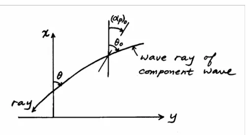
Ray theory for regular waves

Conservation of energy:

0 0 2 0 2

8 1 8

1ρgH C_gb= ρgH C_g b

which gives

r sK K H H = ₀

shoaling coefficient, ( , )

2 sinh 1 2 tanh

2 / 1

0 K f h

kh kh kh

C

K C _s

g g

s ⎥⎦ =

⎢ ⎤

⎣

⎡ ⎟

⎠

⎜ ⎞

⎝⎛ +

=

=

−

refraction coefficient, ⁰ K (f, ,h) b

K_r = b = _r θ ; )θ =θ(f,h,θ₀

3.1.2 Refraction Coefficient of Random Sea Waves

[ ]

θ θ θ θ

θ ∂

= ( , ) ( , , )² ₀( , ₀)∂ ⁰ )

,

(f K f h K f h S f

S _{s r}

[ ] [ ]

0

2 0 0

0

2 ( , ) ( , , )

) , ( )

, ( )

( θ θ ^π θ θ θ

π π

πS f d K f h S f K f h d

f

S =

∫

− = _s

∫

− _r

[ ]

[ ]

∫ ∫

∫ ∫

∫

∞

∞

−

∞

=

=

=

0 0

2 0 0

0

0 0

2 0 0

0 0 0

max min

) , , ( ) , ( ) , (

) , , ( ) , ( ) , ( )

(

df d h f K h f K f S

df d h f K h f K f S df

f S m

r s

r s

θ θ π

π

θ θ θ

θ θ θ

Goda’s book uses

[ ]

∫ ∫

^∞

= 0 0

2 0

0 0

max min

) , ( ) ,

(f K f h d df

S

m_s ^θ _s

θ θ θ

Define

( )

^1/2

0 0 ⎟⎟

⎠

⎜⎜ ⎞

⎝

=⎛

s r eff

m K m

For example, H_m0 =4 m₀ = significant wave height after shoaling and refraction H_ms0 =4 m_s0 = significant wave height due to shoaling only then, Hm0 =

( )

Kr effHms0

Goda’s book explains how to discretize f and θ.

area total )

0 (

0 =

∫

^{∞S f df} = m

) , , 2 , 1 ( )

( ⁰

~

~ i M

M df m f

iS

i

i

f f

f = = L

∫

^+Δ

) (f

S can be integrated analytically (e.g. B-M or P-M spectra), say )

exp(

)

(f =af⁻⁵ −bf⁻⁴ S

b bf a

b df a f S

m exp( ) 4

) 4 (

0 4

0 0 =

⎥⎦⎤

⎢⎣⎡ −

=

=

∞

∞ −

∫

Similarly,

{ }

M f m

b f

f b b

bf a b

df a f

S _{i i i}

f f

f f

f f

i i

i i

i i

4 0 4

~

~ 4

~

~ ~ )

exp(

]

~ ) ( 4 exp[

) 4 exp(

)

( = − +Δ − − =

⎥⎦⎤

⎢⎣⎡ −

= ^{− −}

Δ + Δ −

∫

+

Hence,

) , , 2 , 1 1 (

~ ) exp(

]

~ ) (

exp[ ^{4 4} i M

f M b f

f

b _i+Δ _i − − _i = = L

− ^{− −}

Now we can find Δf_i (i=1,2,L,M) starting from ~ 0.

1= f

Representative frequency f_i for the band (~f_i

to ~f_i +Δf_i )?

Goda suggests on the basis of T = m₀/m₂ and ⁼

∫

0^∞ 2

2 f S(f)df

m

( ) ( )

_iⁱ

i m

f m

0

≅ 2

( )

b M

a M

m _i m 1

4

0

0 = =

( )

⁼

∫

^{+Δ =}

∫

i^{i+Δi − − −} i

i i

f f f f

f

i f f S f df af bf df

m

~

~

4 3

~

~ 2

2 ( ) exp( )

Putting

b df d

f f

b 2 2 2

3 2

= −

→

= ⁻

− ξ ξ

,

( ) ∫

^{− −}

∫

+⁻Δ ⁻

Δ

+ − = −

−

= ₂ ^{2 2 (~) 2} ₂

~ ) ( 2 ) 2

(~ 2

~) ( 2

2

2 exp( /2)

2 ) 2

2 / 2 exp(

2

i i i i

i i

f b

f f b f

f b

f

i b d

b d a

b

m a ξ ξ ξ ξ

Goda defines error function, ^{Φ t =}

∫

0^{t −x dx} 2/2) exp(

2 / 1 )

( π , though usual definition is

∫

⁻

= ^t x dx

t

erf 0

2) exp(

/ 2 )

( π so that erf(∞)=1. Thus,

( )

2 ⁼ _⎩⎨^⎧Φ_⎢⎣^⎡

( )

⁻²_⎥⎦^⎤−Φ_⎢⎣^⎡

(

^+Δ

)

⁻²_⎥⎦^⎤_⎭⎬^⎫

2 ~ 2 ~

2 ^{i i i}

i b f b f f

b

m a π

( ) ( ) ( )1/2 ( )2 ( )2 1/2

0

2 ~

~ 2 2

2 ⎭⎬⎫

⎩⎨⎧

⎥⎦⎤

⎢⎣⎡ +Δ Φ

⎥⎦−

⎢⎣ ⎤ Φ⎡

=

= _i ⁻ _{i i} ⁻

i i

i b M b f b f f

m

f m π

which should correspond to Eq. (3.7) in Goda’s book if b=1.03T_s⁻⁴ (B-M spectrum):

2 / 1 2

/

1 2ln

ln 1 2 )

912 . 2 9 ( . 0

1

⎪⎭

⎪⎬

⎫

⎪⎩

⎪⎨

⎧

⎟⎟⎠

⎞

⎜⎜⎝ Φ⎛

⎟⎟−

⎠

⎞

⎜⎜⎝

⎛ Φ −

= i

M i

M M f T

s i

It is required

( )

^{~ ( 1,2, , )}

1 2 ln

2 b f ² i M

i M

i = L

− =

−

On the other hand,

( ) ( )

f M b f

f

b _{i i} ~_i 1

~ exp

exp ^{4 4}⎥⎦⎤=

⎢⎣⎡−

⎥⎦−

⎢⎣ ⎤

⎡− +Δ ^{− −}

Take

ln 1

~ 4

= −

−

i f M

b_i . Then

M M

i M

i 1⎟= 1

⎠

⎜ ⎞

⎝

−⎛ −

⎟⎠

⎜ ⎞

⎝

⎛ satisfied.

As for the discretization of wave angle θ (16-point bearing, see Table 3.2),

3.1.3 Computation of Random Wave Refraction by Means of the Energy Flux Equation General transport equation for S (any scalar quantity):

Q V t S

S +∇⋅ =

∂

∂ ( ) (sink or source of S)

where V = transport velocity of S. For S(t,x,y,f,θ) = directional random waves,

V = velocity following waves

(

vx vy v vf

)

dt df dt d dt dy dt

V dx, , θ , ₌ , , _θ,

⎟⎠

⎜ ⎞

⎝

=⎛

with

θ

gcos

x C

v = , v_y =C_gsinθ

⎟⎟⎠

⎜⎜ ⎞

⎝

⎛

∂

−∂

∂

= ∂ θ θ

θ sin cos

y C x

C C

v C^g to account for refraction

=0

vf assuming f does not change following the wave.

Then

[ ] [

^{S f v}

] [

^{S f v}

]

^Q

v y f x S t

f S

y

x =

∂ + ∂

∂ + ∂

∂ + ∂

∂

∂

θ θ

θ θ θ θ

) , ( )

, ( )

, ) (

, (

For steady state (∂S/∂t =0) with no sink or source (Q=0),

( ) ( ) ( )

=⁰

∂ + ∂

∂ + ∂

∂

∂

θ ^Svθ

y Sv

x Sv^{x y} for S(x,y,f,θ)

Assuming )θ ≠θ(x,y , or x, y, θ are independent variables,

( ) ( )

0 cos

sin sin

cos ⎟⎟⎠=

⎜⎜ ⎞

⎝

⎛

∂

− ∂

∂

∂

∂ + ∂

∂ + ∂

∂

∂

y C x

C C S

y SCC x

SCC

g g

g θ θ

θ θ θ

where C and C_g using linear wave theory depend on h(x,y) and frequency f . θ is computed by ray theory. We need boundary conditions for S.

Example in Goda’s book Fig. 3.3: Waves over a circular shoal

• T_s as well as H_s changes depending on locations (Fig. 3.4).

• Fig. 3.5 for regular waves shows larger spatial variations of wave heights.

Ref. Vincent and Briggs (1989). Refraction-diffraction of irregular waves over a mound, JWPCOE, 115(2), 269-284: Performed laboratory experiments on transformation of monochromatic and random directional waves over an elliptic shoal. They concluded

that monochromatic waves using representative wave height and period (e.g. and ) provide a poor approximation of irregular wave conditions if there is directional spread or high wave steepness.

Hs

Ts

Ref. 권혁민 (1998). 방향 스펙트럼 파랑에 대한 3 차원 쇄파변형 모델,

대한토목학회논문집, 18(II-6), 591-599: Include sink term due to wave breaking.

Ref. Mase, H. (2001). Multi-directional random wave transformation model based on energy balance equation, Coastal Engineering Journal, 43(4), 317-337: Include wave diffraction.

3.1.4 Wave Refraction on a Coast with Straight, Parallel Depth Contours

Snell’s law:

0

sin 0

sin

C C

θ

θ ₌ → can find θ(f,h,θ₀) → θ0

θ

∂

∂

Refraction coefficient

θ θ θ

cos ) cos , ,

(f h ₀ = ⁰

K_r

Shoaling coefficient ⁰ K (f,h) C

K C _s

g g

s = =

Directional spectrum S(f,θ) in water depth h:

[

^{( , ) ( , , )}

]

^{( , )}

) ,

( _{0 0}

1

0 2

0 θ

θ θ θ

θ K f h K f h S f

f

S _{s r}

−

⎟⎟⎠

⎜⎜ ⎞

⎝

⎛

∂

= ∂

Need to specify S₀(f,θ₀) in deep water. For example, S₀(f,θ₀)=S₀(f)G(f,θ₀) with = B-M spectrum with given S₀(f) H_s =H_m0 and T_s =T_p/1.05,

G(f,θ₀) = Mitsuyasu-type with given s_max and

( )

αp ₀,

( )

αp ₀ = predominant wave direction in deep water, ^{θ θ}

( )

^α _⎥ ^{−π ≤}

[

^{θ −}

( )

^α

]

^≤π

⎦

⎢ ⎤

⎣

= ₀ ² ⎡ −^{0 0} _{0 0}

0 ;

cos 2 )

,

(f G ^{s p} _p

G ,

G=G₀ is maximum at θ0 =

( )

αp ₀.

Fig. 3.6 shows

( )

Kr _eff given by Eq. (3.2) as a function of h/L₀ with L₀ = gT_s²/2π ,

( )

αp ₀ and s_max.

Note:

( )

K_{r eff} ≠1 even for

( )

αp ₀ ⁼⁰ (Q directional spreading).

3.2 Wave Diffraction

3.2.1 Principle of Random Wave Diffraction Analysis

For linear monochromatic waves in constant water depth, Sommerfeld solution for a semi-infinite thin breakwater:

Diffraction coefficient K_d =H(x,y)/H_i depends on f , θ_i, and h=constant.

) , ( )

(

) , ,

; , ( )

, (

i i

i i

d

f S f

S

H h y x f K y x H

θ θ

↓

↓

=

Frequency spectrum

[ ]

∫

−

= ^π

π K_d f θ_i S_i f θ_i dθ_i y

x f

S( ) at given ( , ) ( , )² ( , )

Since

[ ]

∫ ∫

∫ ∫

∫

^∞ −

∞

−

∞ = =

0

2 0

0 ( ) ( , ) ^π ( , ) ( , )

π π

πS f θ dθdf K f θ S f θ dθdf

df f

S _{d i i i i}

therefore

[ ]

θ θ θ θ

θ ∂

= K_d f _i S_i f _i ∂ ⁱ f

S( , ) ( , )² ( , )

Then

[ ]

∫

∫

− = −

= ^π

π π

πS f θ dθ K_d f θ_i S_i f θ_i dθ_i f

S( ) ( , ) ( , )² ( , )

In terms of zeroth moment,

( )

m _i S_i f _i d _idf

(

H_m0

)

_i

( )

m_{0 i}

0 =

∫ ∫

0^∞ − ( , ) → =4

π

π θ θ : incident significant wave height

0 0 0

0 S(f, )d df H 4 m

m =

∫ ∫

^∞ − → _m =

π

π θ θ : significant wave height at (x,y)

[ ]

∫ ∫

^∞ −

= 0

2

0 ^π ( , ) ( , )

π K f θ S f θ dθdf

m _{d i i i i}

Define effective diffraction coefficient:

( ) ( ) ( )

( ) [ ]

^1/2

0

2 0

2 / 1

0 0 0

0

) , ( ) , 1 (

added book where

s Goda' in (3.14)

⎥⎦

⎢ ⎤

⎣

=⎡

⎥ =

⎦

⎢ ⎤

⎣

=⎡

=

∫ ∫

^∞ − π

πS f θ K f θ dθdf

m m i m H

K H

i i d i i i

i m i

m d eff

Read Goda’s book for field measurement (Figs. 3.9 and 3.10).

( )

Kd eff >Kd based on regular waves with H =H_1/3 and T =T_1/3 = 0.07, which is significantly underestimated in this case.

3.2.2 Diffraction Diagrams of Random Sea Waves

[ ]

∫

−

= ^π

π K_d f θ_i x y h S_i f θ_i dθ_i h

y x f

S( ; , , ) ( , ; , , )² ( , )

∫

^∞

= 0

0(x,y,h) S(f)df

m ;

( )

m0 _i ⁼

∫

0^∞S_i(f)df

∫

^∞

= 0 2

2(x,y,h) f S(f)df

m ;

( )

⁼

∫

0^∞

2

2 f S(f)df

m _{i i}

peak from T_p(x,y,h) S(f); peak

( )

Tp _i from S_i(f)

2 0 0

0 4 m , T m /m

H_m = = ;

(

Hm₀

)

i =4

( )

m₀ i,

( )

T i =

( ) ( )

m₀ i/ m₂ i

05 . 1 /

0, s p

m

s H T T

H ≅ ≅ ;

( ) (

H_{s i} ≅ H_m0

) ( )

_i, T_{s i} ≅

( )

T_{p i}/1.05 Wave height ratio =

( ) ( ) ( )

s _i

s m i

m d eff

H H H

K = H ≅

0

0 only for H_m0 =H_s

Period ratio

( )

T i

≅ T or

( ) ( )

s i s p i

p

T T T

T ≅

It is not specified in Goda’s book which relation is used for period ratio. It is likely to use T/

( )

T i since T_p may be difficult to find. But Goda uses

( )

Ts _i to find L (p.59).

Goda assumed S_i(f,θ_i)=S_i(f)G(f,θ_i) with B-M frequency spectrum and Mitsuyasu-type directional spreading.

Need to specify

( ) (

Hs i = Hm₀

)

_i,

( )

T_{s i} =

( )

T_{p i}/1.05, s_max,

( )

αp _i, constant depth , and breakwater geometry.

h

( )

⎪⎩

( )

⎪⎨

⎧

=

=

(probably)

ratio period

ratio height Plotted

s i s d eff

T T K

for normal incidence only,

( )

αp _i ^=0°.

Fig. 3.11 for a semi-infinite breakwater, for s_max =10 (wind waves) and (swell, more unidirectional).

max =75 s

Monochromatic versus directional random waves:

1) In general, monochromatic wave underestimates wave heights in sheltered area, and overestimates in open area.

2) The wave height ratio along the boundary of the geometric shadow (or the straight line from the tip of the breakwater to the wave direction) is 0.7 for directional random waves, while it is 0.5 for monochromatic waves.

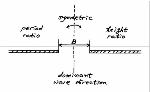
Figs. 3.12~3.15 for breakwater gap (B/L=1,2,4,8)

3.2.3 Random Wave Diffraction of Oblique Incidence

Construct your own computer program if exact solution is needed. Otherwise, use an approximate method suggested in the book.

3.2.4 Approximate Estimation of Diffracted Height by the Angular Spreading Method For large barriers (e.g. headlands and islands),

⎩⎨

⎧

≅

≅

region d illuminate in

1

shadow geometric

in roughly 0

d d

K K

Neglect wave refraction.

( )

=

∫ ∫

^∞ −

0 0 ^π ( , )

πS f θ dθdf

m _{i i i i}

Assume 0S_i = for θ_i >π/2.

( )

=

∫ ∫

^∞ − 0

2 /

2

0 ^π / ( , )

π S f θ dθdf

m _{i i i i}

[ ]

∫ ∫

^∞ −

= 0 2 /

2 /

2

0 ^π ( , ) ( , )

π K f θ S f θ dθdf

m _{d i i i i}

⎩⎨

⎧

≤

<

=

≤

≤

−

=

2 / for

0

2 / for Assume 1

1

1

π θ θ

θ θ π

i d

i d

K K

Then

∫ ∫

^∞ −

= 0 /2 0

1 ( , )

θ

π S f θ dθdf

m _{i i i}

( )

spreading) Mitsuyasu

spectrum M

- (B 2.15 Fig.

or (2.27) Eq.

to 2 / from energy relative

cumulative )

( _{1 1}

0 0

+

=

−

=

= _E θ π θ

i

m P m

( ) ( )

^1/2

[

₁

]

^1/2

0

0 _E(θ )

i

d eff P

m

K m ⎥ =

⎦

⎢ ⎤

⎣

=⎡

1<0

θ and θ₂ >0 for this problem

∫ ∫

∫ ∫

∞

∞

−

+

=

0 2 /

0 /2

0

2 1

) , (

) , (

π θ θ

π

θ θ

θ θ

df d f S

df d f S m

i i i

i i i

( )

( ₁)

[

( /2) ( ₂)

]

0

0 _E θ _E π _E θ

i

P P

m P

m = + −

( ) ( ) [ ]

( ) ( )

^{in the text}

) ( 1 ) (

2 2 2

1

2 1

0 2 0

d d

E E

i d eff

K K

P m P

K m

+

=

− +

=

= θ θ

3.2.5 Applicability of Regular Wave Diffraction Diagrams ↑

Only for very narrow directional spreading

3.3 Equivalent Deepwater Wave

In real situation,

Hydraulic model test in 2D wave flume,

In real situation, Hs =KdKrKsKf

( )

Hs ₀

In 2D wave flume, H_s =K_sH₀' Thus, H0'=K_dK_rK_f

( )

H_{s 0}

↑

(unrefracted) equivalent deepwater wave height

For wave period, usually assumes T_s =

( )

T_{s 0} ← error if diffraction is dominant.

3.4 Wave Shoaling

Linear wave shoaling coeff.

L h C

C H

K H

g g

s function of

'

0 0

=

=

= (3.16)

For shoaling of normally-incident linear random waves,

[

( ; )

]

( ) )

;

(f h K f h ²S₀ f

S = _s ← can write a computer program easily.

For shoaling of nonlinear monochromatic waves, use Shuto (1974) model (read text).

3.5 Wave Deformation Due to Random Breaking

3.5.1 Limiting Wave Height of Regular Waves by Breaking

⎟⎟⎠

⎜⎜ ⎞

⎝

= ⎛

0

, tan L f h

h

H _b

b

b θ → Fig. 3.23

Goda’s empirical formula (1970):

(

⎭⎬⎫

⎩⎨

⎧ ⎥

⎦

⎢ ⎤

⎣

⎡− +

−

= π 4/3θ

0 0

tan 15 1 5 . 1 exp

1 L

A h L

H_{b b}

)

(3.22)

with L₀ =gT²/2π ; A≅0.17

3.5.2 Computational Model of Random Wave Breaking Before wave breaking, Rayleigh distribution may be assumed

H x H x

x x

p ⎟ =

⎠

⎜ ⎞

⎝⎛−

= ;

exp 4 ) 2

( ²

0

π

π (2.1)

After breaking, p₀(x)→ p(x)

1− p_b =probability of non−breaking

⎪⎪

⎩

⎪⎪⎨

⎧

≤

<

− <

− ≥

=

−

2 1 2

2 1

1

1

for 1

for

for 0 1

x x

x x x x

x x x

x x p_b

Let ¹

(

1

)

1 since

0 − 0 <

=

∫

^{x pb p dx}

A 1

0 0 =

∫

^{∞p dx}

Assume p.d.f. adjusted for wave breaking:

(

1

)

( ) ) 1

( p p₀ x

x A

p = − _b so that ( ) 1

0 =

∫

^{∞p x dx}

3.5.3 Computation of the Change in Wave Height Distribution Due to Random Wave Breaking

Need to estimate of wave breaking.

⎭⎬

⎫

⎩⎨

⎧

=

=

limit lower

limit upper

2 1

x x

Use

(

⎭⎬

⎫

⎩⎨

⎧ ⎥

⎦

⎢ ⎤

⎣

⎡− +

−

= π 4/3θ

0 0

tan 15 1 5 . 1 exp

1 L

A h L

H_b

)

(3.22)

with

π 2

2 0

gTs

L = and tanθ = beach slope

⎩⎨

⎧

=

= =

2 1

for 12 . 0

for 18 . 0

x x

x A x

Eq. (3.22) was developed for breaking point (h=h_b) of regular waves. But it may be used inside the surf zone if H_b = broken wave height, h = local depth.

Water level change:

Wave setup (η) was computed using the results of monochromatic waves with T_s and H2 = mean square of random waves, the latter of which is affected by η. Therefore, we need iteration to solve η and H² simultaneously. See Eq. (3.23).

Surf beat, ζ(t): slow (30~300 s) fluctuation of free surface mainly inside surf zone

↑

from Gaussian distribution with ζ_rms given by Eq. (3.24)

Thus, h=d+η+ζ(t)

3.6 Wave Reflection and Dissipation

3.6.1 Coefficient of Wave Reflection

i R

R H

K = H

Typical reflection coefficients are given in Table 3.7.

For perforated wall caissons, becomes minimum (0.3~0.4) at

(see Fig. 3.36). Under a standing wave system, maximum at node → maximum energy dissipation & minimum reflection at

KR B/L=0.15~0.2

u 4

/ L

B= → B/L=0.25. However, in reality, minimum reflection occurs at B/L=0.15~0.2, due to inertia effect.

3.6.2 Propagation of Reflected Waves

r

i θ

θ = (geometrical optics theory) diamond pattern of surface profile

For long-period waves incident at large angle, Mach stem is formed.

amplitude dispersion (Higher waves go faster.) Reflection from finite length of seawall ← diffraction by breakwater gap

Reflection from very long seawall ← diffraction by semi-infinite breakwater (or angular spreading method for headland)

Effect of opposing wind (sea → land): attenuates waves of large steepness, but its effect is minor for swell of low steepness.

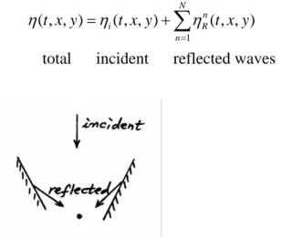
3.6.3 Superposition of Incident and Reflected Waves

For linear waves, we can superpose the free surface displacement:

∑

=

+

= ^N

n n R

i t x y t x y

y x t

1

) , , ( )

, , ( ) , ,

( η η

η

total incident reflected waves

Time-averaged energy per unit surface area:

0 2 at given (x,y) gm

gη ρ

ρ = ; m0 ⁼

∫

0^∞S(f)df

If the distance from the reflective structure is more than one wavelength, we may assume

) ( 0 ),

, , 2 , 1 (

0 n N _Rⁿ _R^m n m

n R

iη = = η η = ≠

η _L uncorrelated.

Then

∑ ( )

=

+

= ^N

n n R i

1 2 2

2 η η

η

( ) ∑ ( )

=

← +

= ^N

n

n R

i m m S(f)

m m

1

0 0

0

0 addition of area under spectrum

( ) ∑ [ ( )

=

+

= ^N

n

n m R m i

m H H

H

1

2 0 2

0 2

0

]

(3.28)

Fig. 3.40 indicates H_m0 ≅

(

H_m0

) (

²_i + H_m0

)

²_R at x/L≥1.0

3.7 Spatial Variation of Wave Height along Reflective Structures

3.7.1 Wave Height Variation near the Tip of a Semi-Infinite Structure

Wave height (crest elevation – trough elevation) along vertical wall (y=0):

2

2 ( )

) 1

(C S C S

H H

I

S = + + + −

where

∫

^⎜_⎝^{⎛ ⎟}_⎠^⎞

= ^u t dt

C

0

2

cos π2

, ^{S =}

∫

0^{u ⎜}_⎝^{⎛ t ⎟}_⎠^⎞dt 2

sin π2

, 2 sin2

2 θ

L u= x

Note: at x=0, u=0 → C=S=0 → H_S/H_I =1 As x→∞, u→∞, then

2

→1 C ,

2

→1

S ∴ =2

I S

H H

less undulation for irregular waves

For irregular waves,

I S

d H

K = H was used in Eq. (3.14)

↑

for component waves ( f →L→u) Explains meandering damage of concrete caissons.

3.7.2 Wave Height Variation at an Inward Corner of Reflective Structures

β π

=2

I S

H

H (3.31)

for = , =2

I S

H π H β

, 4

2 =

=

I S

H π H β

wave height H_S= crest elevation – trough elevation

Same as sum of 4 waves

propagating in 4 different directions

If the length is finite, use a computer program or an approximate method given in Goda’s book.

3.7.3 Wave Height Variation along an Island Breakwater

cause undulation along wall (Fig. 3.46 and 3.47)

If B>>L, may add two waves diffracted from each tip:

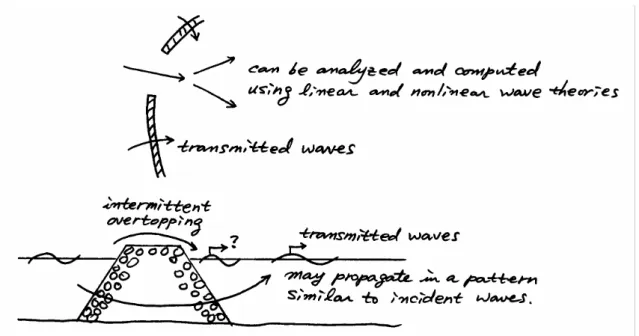
3.8 Wave Transmission over Breakwater

3.8.1 Wave Transmission Coefficient

(A) Vertical breakwater

transmission coefficient

I T

T H

K = H

Wave transmission through rubble mound may be negligible.

Expect _⎟⎟

⎠

⎜⎜ ⎞

⎝

=function⎛ , ,B,T,moundmaterial,L h

d H K h

I c T

Fig. 3.48 for regular wave tests → may be applicable to irregular waves with

and (see Fig. 3.49)

(

_I

I H

H = _1/3

)

HT =

(

H_1/3

)

_T

Eq. (3.33) → _⎟⎟

⎠

⎜⎜ ⎞

⎝

=function⎛ only

I c

T H

K h ; Effect of

h

d is minor (see Fig. 3.48).

Eq. (3.34) → horizontally composite breakwaters

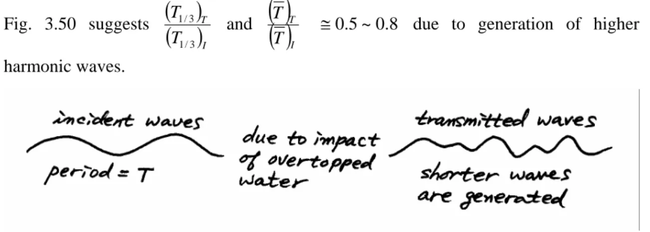
Fig. 3.50 suggests

( ) ( )

T ^T_I

T

3 / 1

3 /

1 and

( ) ( )

I

T

T

T ≅0.5~0.8 due to generation of higher harmonic waves.

(B) Breakwater consisting of energy-dissipating blocks (Tetrapod, Dolos,…) ↓

Fig. 3.51 (C) Rubble mound breakwater

Less void than concrete blocks → smaller K_T (0.1~0.3). But K_T↑ as T↑ 3.8.2 Propagation of Transmitted Waves in a Harbor

No reliable information is available (Read text)

3.9 Longshore Currents by Random Waves on Planar Beach

3.9.1 Longshore Currents by Unidirectional Irregular Waves Longshore current profile for regular waves

Fig. 3.52 gives cross-shore variation of longshore current velocity based on random breaking model discussed in Section 3.5. In terms of deepwater wave condition,

0 0 tan sin velocity

ess dimensionl

α θ gH

v

V = = C^f

0

w.r.t. 0

normalized depth

H H h

z= =

⎥⎥

⎦

⎤

⎢⎢

⎣

⎡ ⎟

⎠

⎜ ⎞

⎝

−⎛ −

⎟⎠

⎜ ⎞

⎝

= ⎛ −

− k

k

A B z A

B v z

z

v( ) exp

1 0

v0, A, B, k are given in Eqs. (3.37) to (3.40) To find v_max,

0 1

exp

exp exp

) 1 (

2 0

1 1

0 2

0

⎪⎭=

⎪⎬

⎫

⎪⎩

⎪⎨

⎧ ⎟

⎠

⎜ ⎞

⎝

− ⎛ −

⎥ −

⎥⎦

⎤

⎢⎢

⎣

⎡ ⎟

⎠

⎜ ⎞

⎝

−⎛ −

⎟⎠

⎜ ⎞

⎝

= ⎛ −

⎥⎥

⎦

⎤

⎢⎢

⎣

⎡ ⎟

⎠

⎜ ⎞

⎝

−⎛ −

⎟⎠

⎜ ⎞

⎝

⎟ ⎛ −

⎠

⎜ ⎞

⎝

− ⎛ −

⎥⎥

⎦

⎤

⎢⎢

⎣

⎡ ⎟

⎠

⎜ ⎞

⎝

−⎛ −

⎟⎠

⎜ ⎞

⎝

− ⎛ −

=

−

−

−

−

k k

k

k k

k k

k

A B k z A k

B z A

B v z

A B z A

B k z A

B v z

A B z A

B k z

dz v dv

−1

⎟ =

⎠

⎜ ⎞

⎝

⎛ − k

A B k z

k

→ A k

B

z ^k 1

1−

⎟ =

⎠

⎜ ⎞

⎝

⎛ − →

k

k A

B

z 1 ^1/

1 ⎟

⎠

⎜ ⎞

⎝⎛ −

− =

→

k

A k B z

/

1 1

1 ⎟

⎠

⎜ ⎞

⎝⎛ − +

=

⎟⎠

⎜ ⎞

⎝⎛ −

⎟⎠

⎜ ⎞

⎝⎛ −

=

∴

−

1 1 1 exp

1

1 1

0

max v k k

v ^k at

k

A k H B

z h

/ 1

0

mode 1

1 ⎟

⎠

⎜ ⎞

⎝⎛ − +

=

= (3.41)

3.9.2 Longshore Currents by Directional Random Waves

smax↓ , more directional spreading, smaller longshore current velocity (see Fig. 3.53).