Chap 3. Generation, Transformation and Deformation of Random Sea Waves

Chap 3. Generation, Transformation and Deformation of Random Sea Waves

3.1 Simplified Forecasting Method of Wind Waves and Swell

Numerical model for directional wave spectrum: WAM or SWAN (including shallow water effects) ← good for both tropical (e.g. typhoon) and extratropical storms

SMB method: Assume a constant wind speed Uover a fixed fetch length F for a certain duration t. Good for extratropical storms (e.g. Northwesters on the west coast of Korea during winter) or wind wave generation in an enclosed basin.

Wilson’s formulas (Eqs. 3.1 and 3.2): Based on SMB method, but modified to be applicable to tropical cyclones of large temporal and spatial variation of wind.

Fully-developed condition: both F and t are long enough Fetch-limited condition: t is long enough, but F is limited Duration-limited condition: F is long enough, but t is limited

Minimum duration for fetch-limited condition = t_min ← Eqs. (3.3) or (3.4)

Minimum fetch length for fully-developed waves for given t = F_min ← Eq. (3.5) If tt_min, fetch-limited → Use Eqs. (3.1) and (3.2)

If tt_min, duration-limited → Calculate F_min using Eq. (3.5). Then use Eqs. (3.1) and (3.2) with F F_min

Relationship between H_1/3 and T_1/3: T_1/3 3.3(H_1/3)^0.63 (3.6) ← good for large waves comparable to design waves but gives lower limit of T_1/3 for smaller waves (see Suh et al. 2010, Coastal Engineering 57, 375-384)

Swell height and period: Eqs. (3.7) and (3.8) as a function of swell travel distance D Relationship between wave height and period of wind waves and swell: Fig. 3.4

3.2 Wave Refraction (+Shoaling)

3.2.1 Introduction

Ray theory for regular waves

Conservation of energy:

0 0 2 0 2

8 1 8

1gH C_gb gH C_g b

which gives

r sK K H H  ₀

shoaling coefficient, ( , )

2 sinh 1 2 tanh

2 / 1

0 K f h

kh kh kh

C

K C _s

g g

s  

 



 



 

 







refraction coefficient, ⁰ K (f, ,h) b

K_r  b  _r  ; ) (f,h,₀

3.2.2 Refraction Coefficient of Random Sea Waves

 



 



 

 ( , ) ( , , )² ₀( , ₀) ⁰ )

,

(f K f h K f h S f

S _{s r}



( , )



² ₀( , ₀)



( , , ₀)



² ₀

) , ( )

(   ^   





S f d K f h S f K f h d

f

S 



  _s



 _r

 

 

 

 

















0 0

2 0 0

0

0 0

2 0 0

0 0 0

max min

) , , ( ) , ( ) , (

) , , ( ) , ( ) , ( )

(

df d h f K h f K f S

df d h f K h f K f S df

f S m

r s

r s





















Goda’s book uses

 

 

^

 0 0

2 0

0 0

max min

) , ( ) ,

(f K f h d df

S

m_s ^ _s

  

Define

 

^1/2

0 0 



 





s r eff

m K m

For example, H_m0 4 m₀ = significant wave height after shoaling and refraction H_ms0 4 m_s0 = significant wave height due to shoaling only then, Hm₀ 

 

Kr effHms₀

In actual calculations, the integration is performed by a summation of frequency and direction.

 

^{2 1/ 2}

1 1

( ) ( )

M N

r eff ij r ij

i j

K E K

 

 





 

Goda’s book explains how to discretize f and .

area total )

0 (

0 



^{S f df}  m

) , , 2 , 1 ( )

( ⁰

~

~ i M

M df m f

iS

i

i

f f

f   



^

) (f

S can be integrated analytically (e.g. B-M or P-M spectra), say )

exp(

)

(f af^5 bf^4 S

b bf a

b df a f S

m exp( ) 4

) 4 (

0 4

0 0 



 







 



Similarly,

 

M f m

b f

f b b

bf a b

df a f

S _{i i i}

f f

f f

f f

i i

i i

i i

4 0 4

~

~ 4

~

~ ~ )

exp(

]

~ ) ( 4 exp[

) 4 exp(

)

(      



 

 ^{ }





 





Hence,

) , , 2 , 1 1 (

~ ) exp(

]

~ ) (

exp[ ^{4 4} i M

f M b f

f

b _i _i   _i   

 ^{ }

Now we can find f_i (i1,2,,M) starting from ~ 0

1 f . Representative frequency f_i for the band (~f_i

to ~f_i f_i )?

Goda suggests on the basis of T  m₀/m₂ and ^



0^ 2

2 f S(f)df

m

   

_iⁱ

i m

f m

0

 2

 

b M

a M

m _i m 1

4

0  0 

 

^



^{ }



i^{ii   } i

i i

f f f f

f

i f f S f df af bf df

m

~

~ 3 4

~

~ 2

2 ( ) exp( )

Putting

b df d

f f

b 2 2 2

3 2

 



 ^

  

,

  

^{ }



^ ^



   



 ₂ ^{2 2 (~) 2} ₂

~ ) ( 2 ) 2

(~ 2

~) ( 2

2

2 exp( /2)

2 ) 2

2 / 2 exp(

2

i i i i

i i

f b

f f b f

f b

f

i b d

b d a

b

m a    

Goda defines error function, ^{ t }



0^{t x dx} 2/2) exp(

2 / 1 )

(  , though usual definition is



^

 ^t x dx

t

erf 0

2) exp(

/ 2 )

(  so that erf()1. Thus,

 

2 ^ _^_^

 

^2_^_^



^



^2_^_^

2 ~ 2 ~

2 ^{i i i}

i b f b f f

b

m a 

     1/2  2  2 1/2

0

2 ~

~ 2 2

2 



 

 





 





 _i ^ _{i i} ^

i i

i b M b f b f f

m

f m 

which should correspond to Eq. (3.15) in Goda’s book if b1.03T_s^4 (B-M spectrum):

2 / 1 2

/

1 2ln

ln 1 2 )

912 . 2 9 ( . 0

1































 

 i

M i

M M f T

s i

It is required

 

^{~ ( 1,2, , )}

1 2 ln

2 b f ² i M

i M

i  

 



On the other hand,

   

f M b f

f

b _{i i} ~_i 1

~ exp

exp ^{4 4}





 

  ^{ }

Take

ln 1

~ ₄

 



i f M

b_i . Then

M M

i M

i 1 1



 



 



 



 satisfied.

As for the discretization of wave angle  (16-point bearing, see Table 3.2),

3.2.3 Computation of Random Wave Refraction by Means of the Energy Balance Equation

General transport equation for S (any scalar quantity):

Q V t S

S  



 ( ) (sink or source of S)

where V = transport velocity of S. For S(t,x,y,f,) = directional random waves,

V = velocity following waves



vx vy v vf



dt df dt d dt dy dt

V dx, ,  , _ , , _,



 





with



gcos

x C

v  , v_y C_gsin



 











   

 sin cos

y C x

C C

v C^g to account for refraction

0

vf assuming f does not change following the wave.

Then

  

^{S f v}

 

^{S f v}



^Q

v y f x S t

f S

y

x 



 



 



 





 

 

 

) , ( )

, ( )

, ) (

, (

For steady state (S/t 0) with no sink or source (Q0),

     

0



 



 





 ^Sv

y Sv

x Sv^{x y} for S(x,y,f,)

Assuming ) (x,y , or x, y,  are independent variables,

 

_sin

 

_{sin cos 0}

cos 

 







 







 



 





y C x

C C S

y SCC x

SCC

g g

g  

 



where C and C_g using linear wave theory depend on h(x,y) and frequency f .  is computed by ray theory. We need boundary conditions for S.

Example in Goda’s book Fig. 3.7: Waves over a circular shoal

• T_s as well as H_s changes depending on locations (Fig. 3.8).

• Fig. 3.9 for regular waves shows larger spatial variations of wave heights.

Ref. Vincent and Briggs (1989). Refraction-diffraction of irregular waves over a mound, JWPCOE, 115(2), 269-284: Performed laboratory experiments on transformation of monochromatic and random directional waves over an elliptic shoal. They concluded that monochromatic waves using representative wave height and period (e.g. H_s and Ts) provide a poor approximation of irregular wave conditions if there is directional spread or high wave steepness.

Ref. Kweon, H.-M. (1998). A 3-D random breaking model for directional spectral waves, Jpornal of the Korean Society of Civil Engineers, 18(II-6), 591-599 (in Korean):

Include sink term due to wave breaking.

Ref. Mase, H. (2001). Multi-directional random wave transformation model based on energy balance equation, Coastal Engineering Journal, 43(4), 317-337: Include wave diffraction.

3.2.4 Wave Refraction on a Coast with Straight, Parallel Depth Contours

Snell’s law:

0

sin 0

sin

C C



 _  can find (f,h,₀) 

0







Refraction coefficient



 

cos ) cos , ,

(f h ₀  ⁰

K_r

Shoaling coefficient ⁰ K (f,h) C

K C _s

g g

s  

Directional spectrum S(f,) in water depth h:



^{( , ) ( , , )}



^{( , )}

) ,

( _{0 0}

1

0 2

0 



 

 K f h K f h S f

f

S _{s r}





 







 

Need to specify S₀(f,₀) in deep water. For example, S₀(f,₀)S₀(f)G(f,₀) with )S₀(f = B-M spectrum with given H_s H_m0 and T_s T_p/1.05,

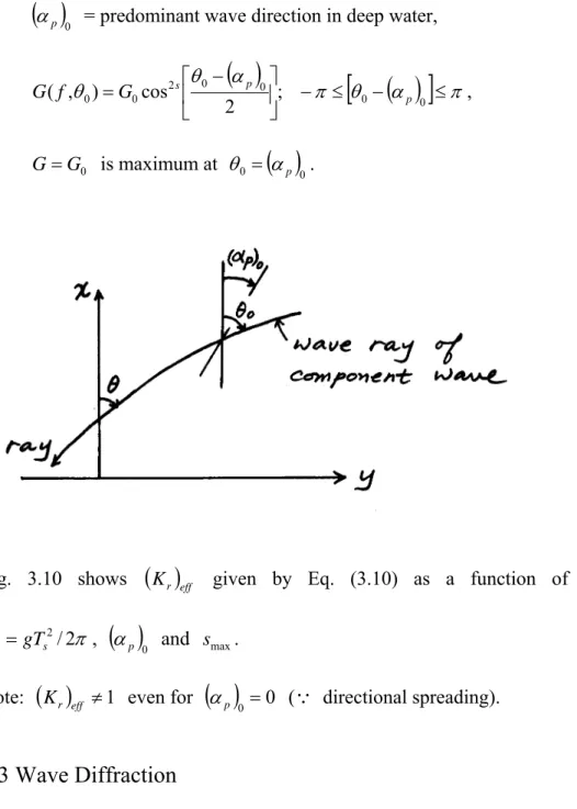
G(f,₀) = Mitsuyasu-type with given s_max and

 

p ₀,

 

p ₀ = predominant wave direction in deep water, ^{ }

 

^ _ ^{ }



^{ }

 

^



^



 



 ₀ ²  ^{0 0} _{0 0}

0 ;

cos 2 )

,

(f G ^{s p} _p

G ,

GG₀ is maximum at ₀ 

 

p ₀.

Fig. 3.10 shows

 

Kr _eff given by Eq. (3.10) as a function of h/L₀ with

 2

2/

0 gTs

L  ,

 

p ₀ and s_max.

Note:

 

K_{r eff} 1 even for

 

p ₀ ^0 ( directional spreading).

3.3 Wave Diffraction

3.3.1 Principle of Random Wave Diffraction Analysis

For linear monochromatic waves in constant water depth, Sommerfeld solution for a semi-infinite thin breakwater:

Diffraction coefficient K_d H(x,y)/H_i depends on f , _i, and h=constant.

) , ( )

(

) , ,

; , ( )

, (

i i

i i

d

f S f

S

H h y x f K y x H











Frequency spectrum

 





 ^

 K_d f _i S_i f _i d_i y

x f

S( ) at given ( , ) ( , )² ( , )

Since

 

 

 



^ 





  

0

2 0

0 ( ) ( , ) ^ ( , ) ( , )





S f  ddf K f  S f  ddf

df f

S _{d i i i i}

therefore

 



 



 

 K_d f _i S_i f _i  ⁱ f

S( , ) ( , )² ( , )

Then

 





  

 ^





S f  d K_d f _i S_i f _i d_i f

S( ) ( , ) ( , )² ( , )

In terms of zeroth moment,

 

m _i S_i f _i d _idf



H_m0



_i

 

m_{0 i}

0 

 

0^  ( , )  4



   : incident significant wave height

0 0 0

0 S(f, )d df H 4 m

m 

 

^   _m 



   : significant wave height at (x,y)

 

 

^ 

 0

2

0 ^ ( , ) ( , )

 K f  S f  ddf

m _{d i i i i}

Define effective diffraction coefficient:

     

   

1/2

0 0

0 0

1/2 2

0 0

(3.22) in Goda's book where added

1 ( , ) ( , )

m d eff

m i i

i i d i i

i

H m

K i

H m

S f K f d df

m



   





 

   

 

 

 

  

 



 



Read Goda’s book for field measurement (Figs. 3.13 and 3.14).

 

Kd eff Kd based on regular waves with H H_1/3 and T T_1/3 = 0.07, which is significantly underestimated in this case.

3.3.2 Diffraction Diagrams of Random Sea Waves

 





 ^

 K_d f _i x y h S_i f _i d_i h

y x f

S( ; , , ) ( , ; , , )² ( , )



^

 0

0(x,y,h) S(f)df

m ;

 

m0 _i ^



0^S_i(f)df



^

 0 2

2(x,y,h) f S(f)df

m ;

 

^



0^

2

2 f S(f)df

m _{i i}

peak )T_p(x,y,h from S(f); peak

 

Tp _i from S_i(f)

2 0 0

0 4 m , T m /m

H_m   ;



Hm₀



i 4

 

m₀ i,

 

T i 

   

m₀ i/ m₂ i

05 . 1 /

0, s p

m

s H T T

H   ;

  

H_{s i}  H_m0

  

_i, T_{s i} 

 

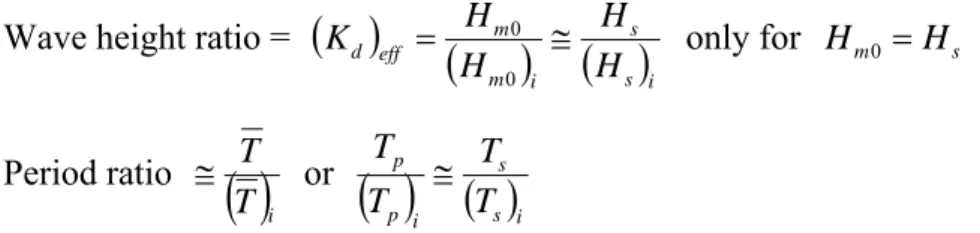
T_{p i}/1.05

Wave height ratio =

     

s _i s m i

m d eff

H H H

K  H 

0

0 only for H_m0 H_s

Period ratio

 

T i

 T or

   

s i s p i

p

T T T

T 

It is not specified in Goda’s book which relation is used for period ratio. It is likely to use T/

 

T i since T_p may be difficult to find. But Goda uses

 

Ts _i to find L (p.82).

Goda assumed S_i(f,_i)S_i(f)G(f,_i) with B-M frequency spectrum and Mitsuyasu-type directional spreading.

Need to specify

  

Hs i  Hm₀



_i,

 

T_{s i} 

 

T_{p i}/1.05, s_max,

 

p _i, constant depth h, and breakwater geometry.

 



 









(probably)

ratio period

ratio height Plotted

s i s d eff

T T K

for normal incidence only,

 

p _i ^0.

Fig. 3.15 for a semi-infinite breakwater, for s_max 10 (wind waves) and s_max 75 (swell, more unidirectional).

Monochromatic versus directional random waves:

1) In general, monochromatic wave underestimates wave heights in sheltered area, and overestimates in open area.

2) The wave height ratio along the boundary of the geometric shadow (or the straight line from the tip of the breakwater to the wave direction) is 0.7 for directional random waves, while it is 0.5 for monochromatic waves.

Figs. 3.16~3.19 for breakwater gap (B/L1,2,4,8)

3.3.3 Random Wave Diffraction of Oblique Incidence

Construct your own computer program if exact solution is needed. Otherwise, use an approximate method suggested in the book.

3.3.4 Approximate Estimation of Diffracted Height by the Angular Spreading Method For large barriers (e.g. headlands and islands),









region d illuminate in

1

shadow geometric

in roughly 0

d d

K K

Neglect wave refraction.

 



 

^ 

0 0 ^ ( , )

S f  ddf

m _{i i i i}

Assume 0S_i  for _i /2.

 



 

^  0

2 /

2

0 ^ / ( , )

 S f  ddf

m _{i i i i}

 

 

^ 

 0 2 /

2 /

2

0 ^ ( , ) ( , )

 K f  S f  ddf

m _{d i i i i}



















2 / for

0

2 / for Assume 1

1

1













i d

i d

K K

Then

 

^ 

 0 /2 0

1 ( , )



 S f  ddf

m _{i i i}

 

0^{0 1 1}

( ) cumulative relative energy from / 2 to

Eq. (2.28) or Fig. 2.15 (B-M spectrum Mitsuyasu spreading)

E i

m P

m     

 

   

^1/2



₁



^1/2

0

0 _E( )

i

d eff P

m

K m  



 





10

 and ₂ 0 for this problem

 

 











0 2 /

0 /2

0

2 1

) , (

) , (

















df d f S

df d f S m

i i i

i i i

 

( ₁)



( /2) ( ₂)



0

0 _E  _E  _E 

i

P P

m P

m   

     

   

in the text ) ( 1 ) (

2 2 2

1

2 1

0 2 0

d d

E E

i d eff

K K

P m P

K m











  

3.3.5 Applicability of Regular Wave Diffraction Diagrams 

Only for very narrow directional spreading

3.4 Equivalent Deepwater Wave

In real situation,

Hydraulic model test in 2D wave flume,

In real situation, Hs KdKrKsKf

 

Hs ₀

In 2D wave flume, H_s K_sH₀' Thus, H₀'K_dK_rK_f

 

H_{s 0}



(unrefracted) equivalent deepwater wave height

For wave period, usually assumes T_s 

 

T_{s 0}  error if diffraction is dominant.

3.5 Wave Shoaling

Linear wave shoaling coeff.

L h C

C H

K H

g g

s function of

'

0 0





 (3.25)

For shoaling of normally-incident linear random waves,



( ; )



( ) )

;

(f h K f h ²S₀ f

S  _s  can write a computer program easily.

For shoaling of nonlinear monochromatic waves, use Shuto (1974) model (read text).

Or you can use Eq. (3.31) with H_1/3 and T_1/3 (see Ex. 3.7).

3.6 Wave Deformation Due to Random Breaking

3.6.1 Breaker Index of Regular Waves

Breaker index:

0

tan ,

b b

b

H h

h f L

   ^  ^

 

Goda’s empirical formula (1970) for regular waves:



^4/3



0 0

1 exp 1.5 1 15 tan ; 0.17

/

b b

b b

H A h

h h L L A

 

  

 

      

  

  (3.32)

with L₀ gT²/2 , which somewhat over-predicts over a steep slope. Rattanapikiton and Shibayama (2000) modified it to



^4/3



0 0

1 exp 1.5 1 11tan ; 0.17

/

b b

b b

H A h

h h L L A

 

  

 

      

  

  (3.33)

3.6.2 Hydrodynamics of Surf Zone

Regular waves break at a fixed location, but random waves break in a wide zone of variable water depth → surf zone

Incipient wave breaking of random waves:

^incipient



^4/3



0 0

0.12 1 exp 1.5 ( )^b 1 11tan

b h

H

L L

 

  

 

     

  

 

Define (h_{1/3 peak}) = water depth at which H_1/3 becomes the maximum inside surf zone,

1/3 peak

(H ) = maximum value of H_1/3 inside surf zone

1/3 peak

(h ) and (H_{1/3 peak}) can be calculated by Figs. 3.28 and 3.29 and Eqs. (3.35)-(3.38).

Incipient breaker index of random waves: (H_{1/3 peak}) / (h_{1/3 peak}) in Fig. 3.30

Distribution of individual wave heights inside surf zone (see Fig. 3.31):

- Rayleigh distribution in relatively deep water

- Enhancement of large waves due to nonlinear shoaling near breaking point → longer right tail

- Breaking of large waves inside surf zone → upper tail truncated

- Regeneration of nonbreaking waves in much shallow area near shoreline → widening toward Rayleigh distribution (not shown in Fig. 3.31)

- Upper curves of Fig. 3.32 (lab, H_2%/H_1/31.4 for Rayleigh) and Fig. 3.33 (field, H_1/10/H_1/3 1.27for Rayleigh) prove these changes.

Water level change:

Wave setup () was computed using the results of monochromatic waves with T_s and H2 = mean square of random waves, the latter of which is affected by . Therefore, we need iteration to solve  and H² simultaneously. See Eq. (3.40) and Fig. 3.34.

 (= at z0) = wave setup at still-water shoreline: Eq. (3.41) and Fig. 3.35

s(maximum ) = maximum wave setup on swash zone: Eq. (3.45)

Surf beat, (t): slow (30~300 s) fluctuation of free surface mainly inside surf zone



from Gaussian distribution with _rms given by Eq. (3.46) Thus, hd (t)

3.6.3 Wave Height Variations on Planar Beaches

Before wave breaking, Rayleigh distribution may be assumed

H x H x

x x

p  



 



 ;

exp 4 ) 2

( ²

0



 (2.1)

After breaking, p₀(x) p(x)

1 p_b probability of nonbreaking













 

 





2 1 2

2 1

1

1

for 1

for

for 0 1

x x

x x x x

x x x

x x p_b

Let ¹



1



1

0  0 





^{x pb p dx}

A since 1

0 0 



^{p dx}

Assume p.d.f. adjusted for wave breaking:



1



( ) ) 1

( p p₀ x

x A

p   _b so that ( ) 1

0 



^{p x dx}

Need to estimate













limit lower

limit upper

2 1

x

x of wave breaking.

Use

 







 



 



 



  4/3

0 0

tan 15 1 5 . 1 exp

1 L

A h L H_b

(3.32)

with

 2

2

0 gTs

L  and tan = beach slope







 

2 1

for 12 . 0

for 18 . 0

x x

x A x

Eq. (3.32) was developed for breaking point (hh_b) of regular waves. But it may be used inside the surf zone if H_b = broken wave height, h = local depth.

Verification of the model with laboratory (Fig. 3.37) and field (Fig. 3.38) data Diagrams (Figs. 3.39 – 3.42) and formulas (Eqs. 3.47 – 3.48 and Table 3.6)

Improved and extended (H_1/3 and H_max → H, H_rms, H_m0, H_1/3, H_1/10 and H_max) equations are given by Rattanapitikon and Shibayama (2013, Coastal Engineering Journal 55(3), 1350009-1~1350009-23)

3.7 Reflection of Waves and Their Propagation and Dissipation

3.7.1 Coefficient of Wave Reflection

R R

I

K H

 H

Typical reflection coefficients are given in Table 3.8.

Reflection coefficient for sloping structure can be calculated by Eq. (3.50).

For perforated wall caissons, K_R becomes minimum (0.3~0.4) at B/L0.15~0.2 (see Fig. 3.44). Under a standing wave system, maximum u at node  maximum energy dissipation & minimum reflection at BL/4  B/L0.25. However, in reality, minimum reflection occurs at B/L0.15~0.2, due to inertia effect.

3.7.2 Propagation of Reflected Waves

r

i 

  (geometrical optics theory) diamond pattern of surface profile

For long-period waves incident at large angle, Mach stem is formed.

amplitude dispersion (Higher waves go faster.)

Reflection from finite length of seawall  diffraction by breakwater gap

Reflection from very long seawall  diffraction by semi-infinite breakwater (or angular spreading method for headland)

Effect of opposing wind (sea  land): attenuates waves of large steepness, but its effect is minor for swell of low steepness.

3.7.3 Superposition of Incident and Reflected Waves

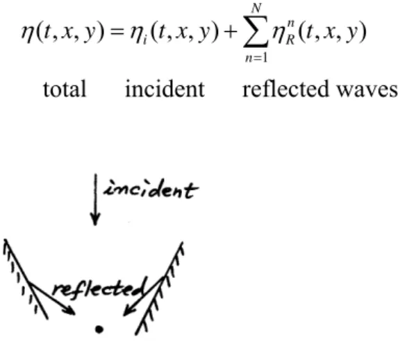
For linear waves, we can superpose the free surface displacement:







 ^N

n n R

i t x y t x y

y x t

1

) , , ( )

, , ( ) , ,

(  



total incident reflected waves

Time-averaged energy per unit surface area:

0 2 at given (x,y) gm

g 

  ; m0 ^



0^S(f)df

If the distance from the reflective structure is more than one wavelength, we may assume

) ( 0 ),

, , 2 , 1 (

0 n N _Rⁿ _R^m n m

n R

i      

  uncorrelated.

Then

  





 ^N

n n R i

1 2 2

2  



    







 ^N

n

n R

i m m S(f)

m m

1 0 0

0

0 addition of area under spectrum

      





 ^N

n

n m R m i

m H H

H

1

2 0 2

0 2

0 (3.51)

Fig. 3.48 indicates H_m0 



H_m0

 

²_i  H_m0



²_R at x L/ 0.7

3.8 Spatial Variation of Wave Height along Reflective Structures

3.8.1 Wave Height Variation near the Tip of a Semi-Infinite Structure

Wave height (crest elevation – trough elevation) along vertical wall (y0):

2

2 ( )

) 1

(C S C S

H H

I

S     

where



^_^{ }_^

 ^u t dt C 0

2

cos 2

, ^{S }



0^{u }_^{ t }_^dt 2

sin 2

, 2 sin2

2 

L u x

Note: at x0, u0  CS0  H_S/H_I 1 As x, u, then

2

1 C ,

2

1

S  2

I S

H H

less undulation for irregular waves

For irregular waves, (K_d)_eff was calculated by Eq. (3.22) with

I S

d H

K  H



for component waves ( f Lu) Explains meandering damage of concrete caissons.

3.8.2 Wave Height Variation at an Inward Corner of Reflective Structures





2

I S

H

H (3.54)

for  , 2

I S

H

 H



, 4

2 



I S

H

 H



wave height H_S= crest elevation – trough elevation

Same as sum of 4 waves

propagating in 4 different directions

If the length is finite, use a computer program or an approximate method given in Goda’s book.

3.8.3 Wave Height Variation along an Island Breakwater

cause undulation along wall (Fig. 3.54 and 3.55)

If BL, may add two waves diffracted from each tip:

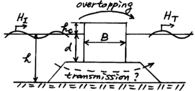
3.9 Wave Transmission at Breakwaters and Low-Crested Structures

3.9.1 Wave Transmission Coefficient of Composite Breakwaters

transmission coefficient

I T

T H

K  H

Wave transmission through rubble mound may be negligible.

Expect _



 



function , ,B,T,moundmaterial, h

d H K h

I c T

Fig. 3.56 for regular wave tests  may be applicable to irregular waves with

 

_I

I H

H  _1/3 and HT 



H_1/3



_T (see Fig. 3.57) Eq. (3.57)  _T function ^c only

si

K h

H

 

  

 ; Effect of h

d is minor (see Fig. 3.56) Eq. (3.58)  horizontally composite breakwaters

1/3 1/3

(T ) / (_T T )_I 1.2K_T 0.28

3.9.2 Wave Transmission Coefficient of Low-Crested Structures (LCS) Low-crested breakwater is built mostly for protection of sandy beaches

Wave transmission through LCS constructed with energy dissipating blocks: Fig. 3.58 (Tetrapods), Eq. (3.59)

Wave transmission over LCS: Eqs. (3.60)-(3.62)

Overall (through+over) transmission of LCS: Eq. (3.63) 3.9.3 Propagation of Transmitted Waves in a Harbor No reliable information is available (Read text)