Introduction
Previous Works
Segmentation algorithm without depth information
- Graph cut
- GrabCut
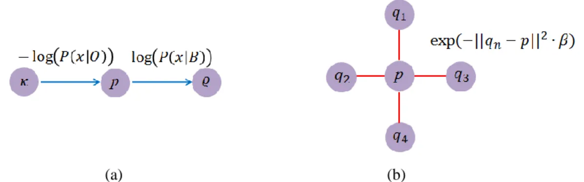
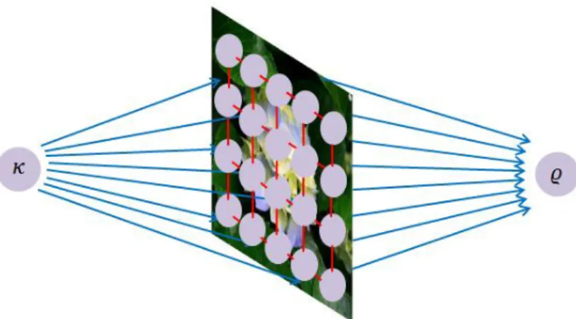
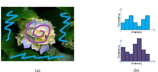
As shown in Figure 2.2, each pixel of an image becomes a node, and there is an edge between neighboring nodes. Since the min-cut/max-flow algorithm behaves like a water flow, it needs a start point 𝜅, which is the origin of the flow, and an end point of the flow 𝜚. After constructing the graph structure, we can add weight to the node and edge to estimate the energy cost of the cut that separates the object from the background.
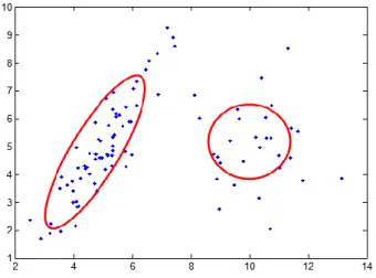
The cost of the energy function 𝐸(𝑋) is determined by the label vector 𝑋 which summarizes each node's labels, including the foreground or background. In the energy function, the smoothness energy function 𝑆 is the summation of the edge costs between pixel nodes. To improve the performance of the Graph cut, GrabCut adopts Gaussian mixture model (GMM) and repeated uses of the min-cut/max-flow algorithm.
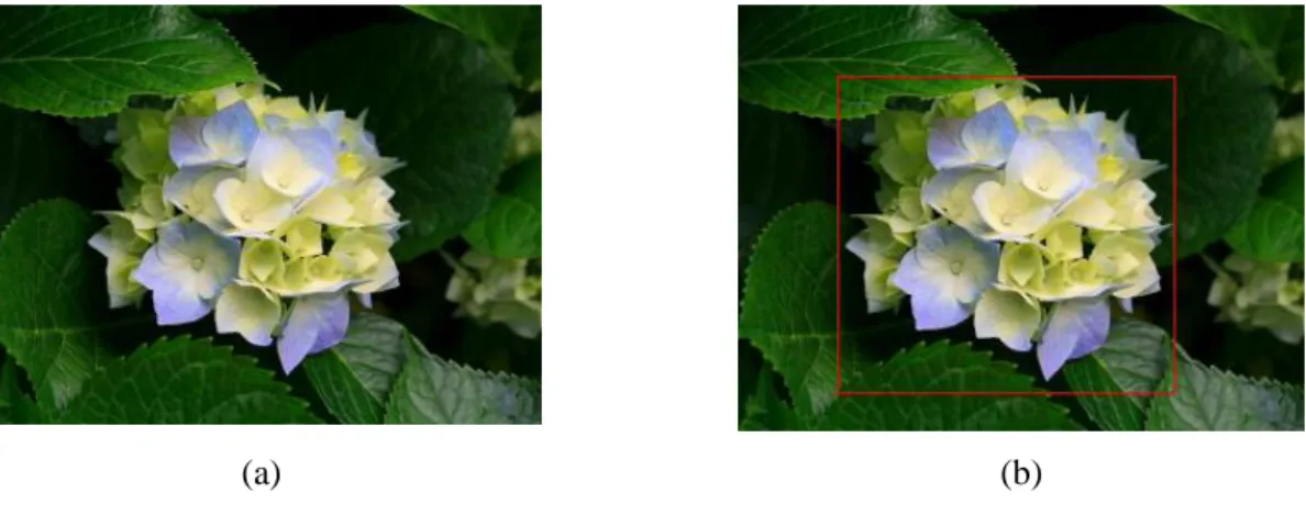
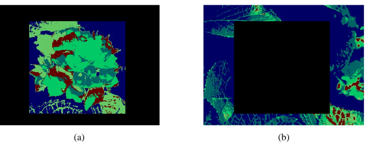
The inside of the bounding box is the foreground, and the outside of the box is the background. After weighting the graph, the method applies the min-cut/max-flow algorithm repeatedly to obtain cuts that separate the object from the image until the flow of the algorithm does not change.
Segmentation algorithm with depth information
- Linearly mixed energy function
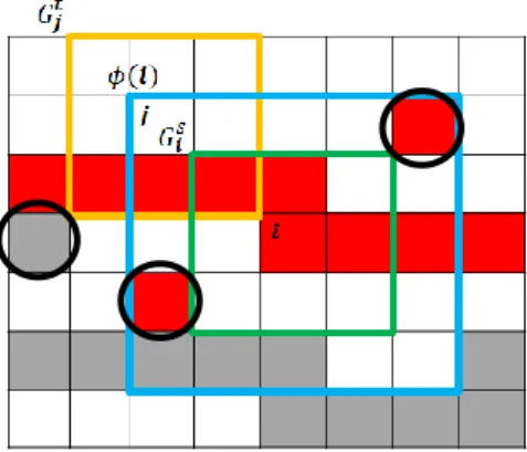
𝐻(𝒙) is the strength of the gradient at 𝒙 in an image, and 𝑃(𝒙) is the value of the grayscale image. As shown in Figure 3.2, to find the best matching position of 𝒊 between color edge pixels, we assign the center of the 3×3 source window 𝐺𝒊𝑠 (green rectangle) at 𝒊 in 𝐻𝑑; and at the same position 𝒊, we set the 5×5 search array 𝜙(𝒊) with 25 positions on 𝐻𝑐 (blue rectangle). The rest of the equation in (3.5) is the same as 𝑁𝐶𝐶 except that it uses 𝑄𝒊𝑠(𝒙) instead of 𝐺𝒊𝑠(𝒙).
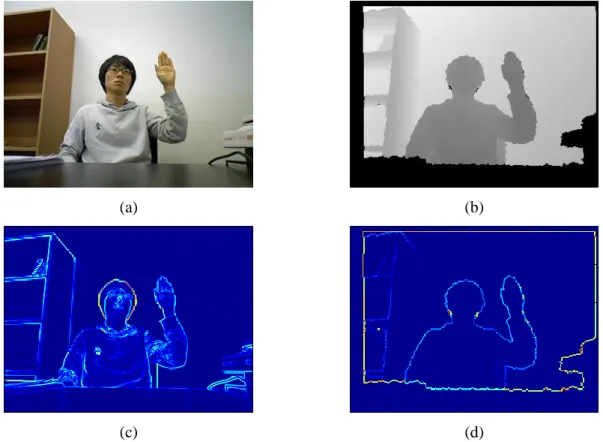
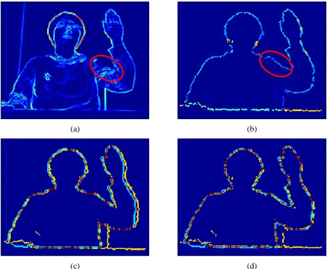
To account for the global motion of the depth edge pixels, we adopt the graph cut of the global optimization algorithm. Using the graph cut result, we can shift the starting positions of the depth edge pixels in the direction of the label field 𝐿. b) Improved depth edges (graph cutting result). Most of the gap caused by the affine transformation error between the color and depth edges is eliminated when we compare the binarized edges in Figure 3.3 (c) with (d).
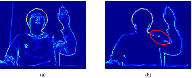
Although the result shows the hidden edges and reduces the gap, some pixels of the refined edges have incorrect values and the shape of the boundary of the color edge object reflects the truth edge values. To take advantage of the refined edges and represent the object boundary well, we need to choose the edges between the color edges and the refined edges. In Figure 3.5 (b), we can see that the edge values are similar to the color edges of Figure 3.5 (a), and these edges exist at the boundary of the object.
Because 𝑈 represents the edges themselves, we can use this 𝑈 value instead of the color difference, as for example below. In the experimental results, we can easily identify the importance of the depth information, as Figure 4.12 shows the difference between GrabCut and the others. In the result of GrabCut, as shown in Figure 4.12 (f), a part of the object has been inverted as background because the object area is very similar to the background colors.
In addition, the algorithm avoids the problem caused by the irregular boundary of the depth image object. Since the depth edges are matched to the color edges, the depth edges of the fake object that are extracted from the background remain in the synthesized edges. In Figure 4.18, because the shape of the object's legs is so complex, our algorithm cannot properly separate the legs.
Proposed Algorithm
Overview
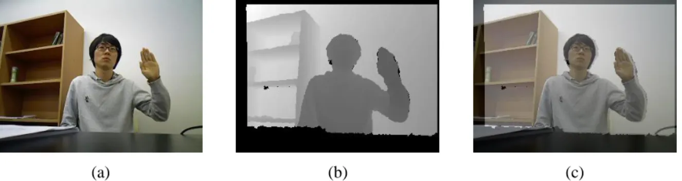
The captured depth image contains significant artifacts near the object boundary, which are caused by affine transformation and device sensor errors. When we use this depth image without any processing to remove these objects, the segmentation result may also have errors. In a depth image, depth edges are drawn out more strongly than in a color image, because the depth image does not have the textures.
However, the depth edge positions are incorrect due to artifacts such as sensor noise. On the other hand, the color edges have the correct positions where the object boundary should be, but there is significant texture noise in the color edges. To combine the individual strengths of the color edges and the depth edges, while eliminating their respective weaknesses, we refine the positions of the depth edges along the color edges using the NCC and graph cut.
Edge extraction
Similarity computation using weighted normalized cross correlation
As a similarity measure, we can use normalized cross-correlation (NCC) because the depth and color images have different pixel values, and the edges derived from them also have different values. However, both source and target windows may have a few outer edge pixels (black circles) away from the main edges, which are the object boundary pixels, so these pixels degrade the performance of NCC. To avoid this problem, we introduce Gaussian weighting to NCC to emphasize the main edge pixels but to reduce the effect of deviant pixels.
NCC is performed by subtracting the mean of edge values and dividing by the standard deviation within each window. 𝐺𝒊𝑠 and 𝐺𝒋𝑡 are the means at each window, and 𝑛 is 9, the number of pixels in the window. 2((𝒙 − 𝜳̅𝒊)𝑇𝚪𝒊−1(𝒙 − 𝜳̅𝒊))) (3.3) 𝑊𝒊𝑠 is the estimated 2-dimensional Gaussian distribution within the source window centered at the gradient window.
Optimal refinement of depth edges using graph cut
𝑄𝒋𝑡(𝒙) also uses the same procedure as 𝑄𝒊𝑠(𝒙) to obtain the result. 3.8) 𝛾𝒊𝑙𝒊 is an element among 𝜸𝒊's elements according to the label value of 𝑙𝒊. To create the result of the refined edges 𝑅, we need to move the initial depth edge pixel positions according to the labels as offset positions and set the values of the edge pixels as the depth. The hidden edges are not extracted from the color edges because the background and foreground colors are similar.
Adaptive edge synthesis
We must select edge points and values between the filled edges 𝐾 and the colored edges 𝐻𝑐 by adaptively using equation (3.11). 𝐾 is close enough to cover the object boundary, but it does not well reflect the object boundary values as the color edges shown in Figure 3.4 (b). To obtain the correct edge values and remove texture noise in Figure 3.4 (b), we take the color edge values instead of the edge values in 𝐾 when the positions of the edge points on 𝐾 are the same as the color edge positions.
When the conditions 𝐾(𝒙) > 0 and 𝐻𝑐(𝒙) > 0 are met, we take the value 𝐻𝑐(𝒙) as a synthesized edge value. Although the color edge 𝐻𝑐(𝒙) does not exist, depth edge 𝐾(𝒙) exists, so we take 𝐾(𝒙) as a hidden edge.
GrabCut-based optimization
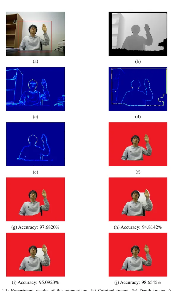
Various object images are used in our experiment to evaluate and compare the proposed algorithm with conventional ones, including GrabCut and the corresponding methods of Hu et al. The size of the search range is ?×?, and the size of the source and target windows is 5 × 5 for refined depth edge searches. On the other hand, in Figure 4.13 (f), the GrabCut algorithm separates the object well because the object has relatively unique colors compared to the background color.
The results of our proposed algorithm show proper segmentation results regardless of the similarity between foreground and background color statistics. In particular, Figure 4.1 (j) shows the effect of synthesized edges when compared to others. In the GrabCut result in Figure 4.1 (g), the upper arm region is misclassified because it has hidden edges, as shown in Figure 3.5 (b);.
The reason for this is that our synthesized edges can effectively find the boundaries of an object without the boundary of a background object such as a whiteboard. First, we manually generate the underlying real object regions and extract the false background and false foreground pixels among 11 test images using algorithm results including those of GrabCut, Hu et al., Vaiapury et al., and our proposed algorithm. Equation (5.1) shows how to calculate the accuracy. where 𝑍 is the number of bounding box pixels, and 𝐹 and 𝐴 are the number of false background and false foreground pixels, respectively.
In this thesis, we proposed an adaptive edge synthesis algorithm for selecting edges between the refined depth edges and the color edges. We first consider the features of the extracted edges from the color image and the depth image. Furthermore, we synthesize the final edges by adaptively selecting the refined depth edge pixels and the color edge pixels.
The experimental results show that the synthesized edges are correctly selected and that the object boundary is maintained relatively well compared to the conventional algorithms. Also, the object can be extracted even if the foreground and background color statistics are the same.
Experimental Results
Conclusion