저작자표시-비영리-변경금지 2.0 대한민국 이용자는 아래의 조건을 따르는 경우에 한하여 자유롭게
l 이 저작물을 복제, 배포, 전송, 전시, 공연 및 방송할 수 있습니다. 다음과 같은 조건을 따라야 합니다:
l 귀하는, 이 저작물의 재이용이나 배포의 경우, 이 저작물에 적용된 이용허락조건 을 명확하게 나타내어야 합니다.
l 저작권자로부터 별도의 허가를 받으면 이러한 조건들은 적용되지 않습니다.
저작권법에 따른 이용자의 권리는 위의 내용에 의하여 영향을 받지 않습니다. 이것은 이용허락규약(Legal Code)을 이해하기 쉽게 요약한 것입니다.
Disclaimer
저작자표시. 귀하는 원저작자를 표시하여야 합니다.
비영리. 귀하는 이 저작물을 영리 목적으로 이용할 수 없습니다.
변경금지. 귀하는 이 저작물을 개작, 변형 또는 가공할 수 없습니다.
공학석사 학위논문
심층 합성곱 신경망 기반의 알츠하이머 생쥐 모델에서 공간 정규화 과정이 필요 없는 표준판 기반 개별 뇌 PET
관심 부피영역 생성 방법
Template-based individual brain PET volumes of interest generation method using deep convolutional neural network without spatial
normalization in mouse Alzheimer's models
울산대학교대학원 의 학 과
서 승 연
Template-based individual brain PET volumes of interest generation method using deep convolutional neural network
without spatial normalization in mouse Alzheimer's models
지도교수 주 세 경 오 정 수
이 논문을 공학석사학위 논문으로 제출함
2022 년 6 월
울 산 대 학 교 대 학 원 의 학 과
서 승 연
서승연의 공학석사학위 논문을 인준함
심사위원 김 재 승 ( 인 ) 심사위원 이 동 윤 ( 인 ) 심사위원 오 정 수 ( 인 )
울 산 대 학교 대 학 원
2022 년 6 월
I. Abstract
PurposeAlthough skull-stripping and brain region segmentation are essential for precise quantitative analysis of positron emission tomography (PET) of mouse brains, deep learning-based unified solutions, particularly for spatial normalization, have posed a challenging problem in deep learning-based image processing. In addition, routine preclinical/clinical PET images cannot always afford corresponding MR and relevant VOIs. In this study, we propose an approach based on deep learning to resolve these issues. We generated both skull-stripping masks and individual-brain-specific volumes-of- interest (VOIs – cortex, hippocampus, striatum, thalamus, and cerebellum) based on inverse-spatial-normalization (iSN) and deep convolutional neural network (deep CNN) models. Furthermore, based on the aforementioned methods, we directly generated target VOIs from18F-fluoro-deoxyglucose positron emission tomography (18F-FDG PET) images not using MR but using only PET images.
Materials and methodsWe applied our devised our devised methods to mutated amyloid precursor protein and presenilin-1 mouse model of Alzheimer’s disease. Eighteen mice underwent T2-weighted MRI and 18F-FDG PET scans twice, before and after the administration of human immunoglobin or antibody-based treatments. For training the CNN, manually-traced brain masks and iSN-based target VOIs were used as the label. For model performance evaluation, DSC, ASSD, SEN, SPE, and PPV between deep learning label mask and deep learning generation mask was evaluated, and the correlation of mean counts and SUVR using each mask (DL-generated mask, DL label mask (i.e., inversely normalized template (ground-truth) VOIs), and template-based ground-truth VOI) was compared.
Results In visual assessment, our deep CNN-based method not only successfully generated brain parenchymal tissue masks and target VOIs using MR images, but also successfully generated target VOIs even when using PET images alone. In addition, both mean counts and SUVRs obtained in the target VOIs (i.e., cortex, hippocampus, striatum, thalamus, and cerebellum) showed significant concordance correlation (CCC > 0.97, P<0.001) in both methods using MR or using only PET.
ConclusionWe propose an unified deep CNN-based model that can generate mouse brain parenchymal masks and inversely-normalized VOI (iVOI) templates in individual brain spaces without extensive efforts for skull-stripping and spatial normalization. We further implemented a new deep CNN-based model based on PET images only to generate iVOI templates. Our devised methods demonstrated the concordant quantification results as compared with the ground- truth method, i.e., spatial normalization and VOI template-based quantification in terms of mean counts and SUVRs in
target VOIs. In conclusion, we established a novel deep leaning-based method for MR template-based VOI generation in an SN-less fashion for PET image quantification.
Contents
I. Abstract
II. List of Table, Figures 1 Introduction
2 Materials and Methods 2.1 Data
2.2 Preprocessing 2.3 Deep CNN
2.4 Performance Evaluation 3 Results
3.1 Deep CNN for automatic generation of brain mask for skull-stripping
3.2 Deep CNN for automatic generation of iVOI template in individual brain space using MR
3.3 Deep CNN for automatic generation of iVOI template in individual brain space using only PET images 4 Discussions
5 Conclusion 6 References 7 Korean Abstract
II. List of Tables.
Table 1. Performance metrics of our unified deep neural network using MR.
Table 2. Performance metrics of our only-PET-based deep neural network.
III. List of Figures.
Figure 1. Schematic diagram of our devised deep CNN model.
Figure 2. Representative samples of deep CNN results for automatic generation of brain masks for skull-stripping using MR.
Figure 3. Representative samples of deep CNN results for automatic generation of target VOIs (i.e., cortex, hippocampus, striatum, thalamus, and cerebellum) using MR.
Figure 4. Scatter plots between all mean counts of radioactivity counts obtained using VOIDL, VOIiGT, and VOIGTin all target VOIs (i.e., cortex, hippocampus, striatum, thalamus, and cerebellum) using MR.
Figure 5. Scatter plots between all SUVR values obtained using VOIDL, VOIiGT, and VOIGTin all target VOIs (i.e., cortex, hippocampus, striatum, and thalamus) using MR.
Figure 6. Bland-Altman plots are depicted to show the difference between all mean counts of radioactivity counts obtained using VOIDL, VOIiGT, and VOIGTin all target VOIs (i.e., cortex, hippocampus, striatum, thalamus, and cerebellum) using MR.
Figure 7. Bland-Altman plots are depicted to show the difference between all SUVR values obtained using VOIDL, VOIiGT, and VOIGTin all target VOIs (i.e., cortex, hippocampus, striatum, and thalamus) using MR.
Figure 8. Representative samples of deep CNN results for automatic generation of target VOIs (i.e., cortex, hippocampus, striatum, thalamus, and cerebellum) using PET.
Figure 9. Scatter plot between all mean counts of radioactivity counts obtained using VOIDL, VOIiGT, and VOIGTin all target VOIs (i.e., cortex, hippocampus, striatum, thalamus, and cerebellum) using PET.
Figure 10. Scatter plots between all SUVR values obtained using VOIDL, VOIiGT, and VOIGTin all target VOIs (i.e., cortex, hippocampus, striatum, and thalamus) using PET.
Figure 11. Bland-Altman plots are depicted to show the difference between all mean counts of radioactivity counts obtained using VOIDL, VOIiGT, and VOIGTin all target VOIs (i.e., cortex, hippocampus, striatum, thalamus, and cerebellum) using PET.
Figure 12. Bland-Altman plots are depicted to show the difference between all SUVR values obtained using VOIDL, VOIiGT, and VOIGTin all target VOIs (i.e., cortex, hippocampus, striatum, and thalamus) using PET.
1 Introduction
18F-fluoro-deoxyglucose positron emission tomography (18F-FDG PET) is a useful imaging technique that enables the investigation of glucose metabolism-based functional imaging not only in human brains but also in mouse brains [1, 2].
Because mouse brains have different shapes and sizes, spatial normalization (SN) of individual brain PET and/or magnetic resonance imaging (MRI) onto standard anatomical spaces is required for objective statistical evaluation [3]. Moreover, we can apply common volume-of-interest (VOI) templates for spatially-normalized individual brain PET and MR images, which can be directly used without labor-intensive manual tracing, and further, can define individual brain-specific VOIs using inverse transformation of SN.
In some human brain studies, the template used for SN was skull-stripped to avoid potential spatial
misregistration due to soft tissues around skulls and brains [4]. Because most mouse brain templates have been based on skull-stripped images, skull-stripping has been considered a prerequisite for the SN of mouse brain MRI and/or PET images [5, 6].
Template-based (also known as atlas-based) brain skull-stripping and brain VOI segmentation methods in mouse brain MRIs have shown accurate segmentation performance in previous studies [6, 7]. In these studies, PET or MRI images of individual brains were registered onto predefined templates of average mouse brains using affine
transformations, occasionally followed by nonlinear registration for more precise registration of the individual brains onto brain templates. Subsequently, the template-based skull-stripped brains were used as starting (or seeding) points to define the individual brain skull-stripping and segmentation. Although these methods were relatively accurate, most of them were conducted semiautomatically, not only resulting in SN with reduced reliability due to inter- and intra-rater reliability issues [8, 9] but also involving time-consuming processes.
Recently, many deep learning (DL)-based skull-stripping methods have been exploited. Hsu et al. (2020) [10]
devised a DL-based framework to automatically identify mouse brains in MR images. The brain mask was generated using randomly-cropped MR image patches as input of the 2D U-Net architecture. For the evaluation of the model, a manually-traced brain mask by an expert and a brain mask generated by the model were evaluated by Dice coefficient and Jaccard index as well as positive predictive value, and sensitivity, and the results showed better performance than conventional methods [11-13]. Similarly, De Feo et al. (2021) [14] proposed Multi-task U-Net (MU-Net) to accomplish skull-stripping and region segmentation. 128 T2-weighted MR images (32 mice x 4 different ages) were used as inputs to
perform the training and validation of their proposed model, and five manually-traced region consisting of cortical, hippocampus, ventricular, striatum and brain masks were used as labels. They demonstrated that MU-Net was able to effectively reduce the inter- and intra-rater variability that occurs when skull-stripping and region segmentation are performed manually and showed better performance than the latest multi-atlas segmentation methods [15, 16].
By contrast, DL-based SN has been a very challenging problem involving many DL-based medical image preprocessing steps. Recently, an interesting DL-based pseudoPET template generation method (as the preprocessing of amyloid PET SN) has been developed using a convolutional autoencoder and a generative adversarial network [17].
Nonetheless, this class of methods commonly generates a pseudotemplate that is a linearly- or nonlinearly-registered individual brain onto the template using a convolutional neural network (CNN), instead of estimating the actual spatial transformations of the individual images onto the template, inevitably requiring additional efforts for the final SN.
Another class of CNN-based spatial registration methods called spatial transformer networks (STNs [18]) has been developed. However, most of them are demonstrated as 2D registration and linear (rigid body or affine) transformation tools. Although a diffeomorphic transformer network was recently developed by Detlefsen et al. (2018) [19] using a continuous piecewise affine transformation, its validation study as an SN tool for PET or MR images has not been conducted thus far. Notably, a DL model-based SN of Tau PET has been developed, which repeatedly estimates sets of rigid and affine transformations using a cascaded set of CNNs [20]. Although rigid and affine transformations have been implemented and evaluated, a non-rigid deformation has not been. Moreover, this class of methods requires a
complicated CNN architecture consisting of cascades of many regression and spatial transformer layers, i.e., numerous CNN parameters to be estimated. This reduces the clinical feasibility of these methods in that considerable amounts of data are required for effective training. Taken together, thus far the SN problem in isolation has not been fully resolved, even in recent DL-based literature, including not only image segmentation [6, 7, 21, and 22] but also apparently more challenging image generation methods, such as PET-based MR generation, to support SN [23].
Considering that DL-based image generation can resolve these challenging issues of medical image preprocessing, we were motivated to reformulate the challenging SN problem into a more easily tractable image generation problem of VOI segmentation. To bridge SN and segmentation, we used the useful approach of iSN. The iSN process involves the operation of generating the inverse of a deformation field and resampling a spatially-normalized image back to the original space (i.e., an individual brain space — [24]). Indeed, we can generate inversely-normalized VOIs (iVOIs) in an individual brain space by applying the iSN technique to VOI templates, as performed in many
neuroimaging studies. Representatively, neuroimage analysis tools such as MarsBar and the Statistical Parametric Mapping (SPM) deformation toolbox conduct iSN-based VOI analysis in an individual (native) brain space and have been frequently used in many brain PET quantification studies [25-27]. Specifically, computed tomography (CT)-based SN was used for 18F-fluoro-propyl-carbomethoxy-iodophenyl-tropane (18F-FP-CIT) PET analysis using an inverse- transformed automatic anatomical label (AAL) VOI template in a couple of previous studies [26, 27].
Inspired by these concepts, we developed a new method for generating the iVOI labels of a deep CNN in an individual brain space. Consequently, we could reduce the abovementioned complicated problem of SN for the final VOI quantification into a much simpler problem of VOI segmentation in an individual brain space that is straightforwardly implemented by modern deep CNNs such as U-Net.
Recently, individual-brain-specific VOI generation methods such as the FreeSurfer software [28], which can produce highly concordant VOIs with respect to manually-traced ground-truth VOIs, have been frequently used in many neuroimaging studies. By contrast, template-based VOI approaches such as SPM present better or equal performance than individual-brain-space VOIs in terms of test–retest reproducibility [29]. Considering this information, our previous iSN- based template VOI defined in the individual brain space leverages the strengths of both methods. Employing the iSN method, we can avoid image deformation, whose magnitude can be described using the Jacobian determinant of the deformation fields [30] and which can lead to differences between the effective voxel sizes of PET images in individual brain and template spaces.
In this regard, herein, we propose both unified deep CNN framework, based on MR or only PET, designed to conduct not only mouse brain parenchyma segmentation (i.e., skull-stripping) but also to generate target VOIs (i.e., cortex, hippocampus, striatum, thalamus, and cerebellum) in an individual brain space. This is achieved using VOI templates defined in mouse MR or PET templates without SN onto a template to facilitate automatic precision 18F-FDG PET analysis with MR-based iVOI using deep CNN. Consequently, we could reduce the relatively complicated brain VOI generation (by skull-stripping and SN) for precise PET quantification to a more tractable problem of DL-based iVOI segmentation in an individual brain space without conducting SN. This approach can avoid the complicated preprocessing steps for skull-stripping and SN for target VOI generation, preventing the unwanted time-consuming process of
semiautomatic skull-stripping and reducing the inter- and intra-rater reliability issues. In addition, our DL-based method can perform precise PET image analysis without a network of complicated structures for SN [20]. In an extended approach for more practical PET image quantitation considering the actual clinical/preclinical practice where MR images
corresponding to PET images were not always expected, we also developed a deep CNN method that could generate iVOI directly from the PET image. Finally, we could establish a new deep CNN-based framework for 18F-FDG PET quantitation by generating iVOI with neither SN nor MR.
2 Materials and Methods
2.1 Data
Eighteen transgenic mice expressing an amyloid precursor protein (APP) and presenilin (PS)-1 Alzheimer’s disease (AD) mouse model underwent brain 18F-FDG PET and T2-weighted MR imaging twice, before (at the age of 9 months) and after the administration of human immunoglobin or antibody-based treatments (at the age of 10 months). The PET images were acquired by nanoScan PET/MRI 1 Tesla (nanoPM – Mediso Medical Imaging Systems, Budapest, Hungary).
Eighteen mice were anesthetized with isoflurane (1.5–2%) and received an intravenous injection of 18F-FDG (0.15 m Ci/0.2 cc). After the acquisition of T2-weighted fast spin echo MRI by nanoPM, the PET static images were acquired for 20 min in list mode and were reconstructed using the ordered-subset maximum-likelihood algorithm using the
abovementioned T2-weighted MR-based attenuation correction in the Nucline software (Reinvent Systems For Science &
Discovery, Mundolsheim, France) in the following parameters—energy window: 250–750 keV; coincidence mode: 1–3;
Tera-tomo3D full detector; regularization: normal; iteration x subset: 8 x 6; voxel size: 0.4 mm. The MR images were acquired using a Bruker 7.0T MRI Small Animal Scanner (Bruker, Massachusetts, United States) reconstruction options of T2-weighted MR images were as follows—repetition time: 4500 ms; echo time: 38.52 ms; field of view (FOV): 20 x 20 mm; slice thickness: 0.8 mm; matrix: 256 x 256; respiration gating was applied.
2.2 Preprocessing
All image preprocessing was performed using SPM 12 software (SPM12; Wellcome Trust Centre for Neuroimaging, London, UK) implemented in MATLAB R2018a (The MathWorks Inc.) and MRIcro (Chris Rorden, Columbia, South Carolina, Unites States). First, the acquired T2-weighted MR images and 18F-FDG PET images were converted from DICOM format to analyze format using MRIcro. PET images were coregistered onto MR images to match different FOVs and slice thicknesses. For brain parenchyma mask generation DL, the entire mouse brain was manually-traced using in-house software (Asan Medical Center Nuclear Medicine Toolkit for Image Quantification of Excellence –
ANTIQUE) [32]. To achieve a more precise SN of the PET image, deformation fields generated by spatial normalizing T2-weighted MR images to the T2-weighted MR template were applied to the corresponding PET images. In addition, to obtain a label image of the “iVOI template” (i.e., VOI template-based and iSN-based VOIs in an individual brain space) generation model, an inverse deformation field was generated and resampled from the VOI template space to the individual image space. This was achieved using the deformation toolbox of SPM, by performing inverse transformation of the deformation fields that map the individual brains onto the template brain. A quantitative evaluation of the PET images by a VOI template was used as the gold standard.
2.3 Deep CNN
A CNN is a deep learning model that enables training while maintaining spatial information, and thus, allows efficient learning with a lighter architecture than a conventional neural network architecture, i.e., fully connected network. For image feature extraction in a CNN, the filters (also known as kernels) in the convolution layers transform the input images into convolution-based filtered output images, termed feature maps. F represents a feature map and is calculated using the following equation:
[ , ] = ( ∗ )[ , ] = [ , ] [ − , − ]
Where represents the input image, represents a kernel, and and represent the index of the rows and columns of the resulting matrix, respectively. For each convolution layer, the shape of the output data is changed according to the filter size, stride, and max pooling size and if zero-padding is applied or not. In this study, we used a quasi-3D U-Net for the deep CNN architecture and an input comprising three consecutive slices for the T2-weighted MR images to generate a brain mask for skull-stripping and an iVOI template in an individual space, as illustrated in Figure 1. Specifically, we used three consecutive slice-based multichannel inputs for the generation of each VOI slice; this 2D-like approach can generate as large amount of training data, as a 2D approach (see Supplementary Material for the comparison of the results of the quasi-3D and 2D approaches). We believe that such an approach can additionally overcome the limitations of the small amounts of mouse data. Moreover, the consecutive slice-based information allows the U-Net architecture to generate a highly continuous VOI by referring to the information of contiguous slices. U-Net consists of an end-to-end CNN architecture using a contracting path of the images and an expanding path for localization and residual learning of images to output layers. The contraction path consists of a 3 × 3 convolution followed by a 2 × 2 max pooling using a
leaky rectified linear unit (leaky ReLU) as the activation function. The expansion path consists of a 2 × 2 deconvolution for upsampling and a 3 × 3 convolution using a leaky ReLU after concatenating with the context captured in the contraction path to increase the accuracy of localization. To train a DL CNN for skull-stripping mask generation, the abovementioned consecutive axial slices of T2-weighted MR images were used as multi-channel input and manually- traced binary brain masks were used as labels. A similar qausi-3D approach was also used in the training of iVOI template generation model, where an iVOI template in an individual space was used as the label. As the U-Net input, the skull-stripping mask generation model and the iVOI template generation model used 70 slices of transaxial MR and the corresponding skull-stripped MR, respectively, and the input dimension was (70 slices × N, 128, 128, 5 channel), where N is the number of mice used in the training set.
To overcome the small amount of data available for training set, data augmentation was performed through shift, rotation, and shear transformations. We used a Dice loss function and an adaptive moment estimation (Adam) optimizer to fit deep CNN parameters. The training was performed with an initial learning rate of 1e-5 with 25 batches.
Our deep CNN model was implemented using Keras (version 2.6.0)-based code in the Python programming language with a backbone of TensorFlow (version 2.6.0) running on a GeForce NVIDIA RTX 3090 GPU and an AMD Ryzen Threadripper 3970X 32-Core Processor CPU. To regularize the generated mask by the deep CNN, we conducted post- processing in several steps, different from other studies that used complicated post-processing methods such as graph cuts [33-35]. First, the mask predicted by deep learning was converted into a binary mask, and erosion and dilation were sequentially performed (also known as the “open” operator) to remove noisy false positives. Subsequently, 3D-connected component analysis-based kill-islands and fill-holes were conducted to reduce false positives and false negatives, respectively
Figure 1
2.4 Performance Evaluation
In order to avoid overfitting issue as well as to increase the generalization ability of the deep CNN, we conducted 6-fold cross-validation for training and test set separation. Of a total 36 samples obtained by 2 scans before and after treatment in 18 mice, 30 samples (15 mice × 2 scans) were used as the training set. The remaining 6 samples (3 mice × 2 scans) were used as the testing set in each fold of the training/test set pair to ensure that the slices of the same mouse are not split as training/test samples. To assess the concordance between predicted and label masks, we measured the Dice similarity coefficient (DSC), average symmetric surface distance (ASSD), sensitivity (SEN), and positive predictive value (PPV).
DSC is the most representative indicator used for image segmentation evaluation. It directly compares the results of the two image segmentations, indicating their similarity. The average symmetrical surface distance is the average of all distances from a point at the boundary of the machine segment region to the boundary of the ground truth. The SEN is defined as the proportion of true positive (TP) results among true positive and false negative (FN). The SPE is defined as the proportion of true negative (TN) among true negative and false positive (FP). PPV is defined as the proportion of true positive among true positive and false positive. Formulas are provided for the five methods as follows, where P is the predicted mask of our network, and G is the label used in deep CNN (See the following equations for the details).
=
| | | || ∩ |,=
∑ ∈ ( ) ∈ ( )‖| ( )| | ( )|‖ ∑ ∈ ( ) ∈ ( )‖ ‖=
,=
,=
.The consistency of PET quantitation between the DL-generated masks and the label masks used in training was evaluated by comparing the mean of radioactivity counts [Bq/mL] estimated by both methods. In addition, uptake ratio, which is also known as standardized uptake value ratio (SUVR) – the most representative and simple method used in the quantitative analysis of 18F-FDG PET used for regional comparison not only between subjects but also within subjects,
was also conducted. In this study, the SUVR analysis was conducted in four major VOIs (i.e., cortex, hippocampus, thalamus, and striatum), and the cerebellum was selected as a reference area since it is the most representative reference region that have relatively intact glucose metabolism in the AD mouse model. The equation for SUVR is as follows.
=
,,
= .
To assess our DL-based method, mean count and SUVR were calculated by the following three different methods: DL-generated mask (VOIDL), DL label mask (i.e., inversely-normalized template (ground-truth) VOIs, VOIiGT), and template-based ground-truth VOI (VOIGT) by scatter plots and Bland-Altman plots (Figure 4-7, and 9-12). Then, correlation analysis was conducted between these methods.
3 Results
3.1 Deep CNN for automatic generation of brain mask for skull-stripping.
Figure 2 shows the comparisons in the brain skull-stripping mask generated by our devised deep CNN (i.e., U-Net) (red contour) and a manually-traced brain mask (blue contour) in three mice. All three mice showed high visual consistency without significant differences.
Table 1 shows the concordance of brain masks generated by a deep CNN and manually-traced masks in terms of the DSC, ASSD, SEN, SPE, and PPV. Mean DSC reached 0.97, mean ASSD was less than 0.01 mm, and mean SEN reached 0.92. In addition, both mean SPE and mean PPV were greater than 0.99. In summary, there was no significant difference between the brain mask generated by our DL-based method and the manually-traced mask in the 6-fold cross- validation.
Figure 2
3.2 Deep CNN for automatic generation of iVOI template in individual brain space using MR.
Figure 3 shows axial slices of VOIDL(blue contour) and VOIiGT(red contour) in target VOIs (cortex, hippocampus, stratum, thalamus and cerebellum). There was no significant difference between VOIDLand VOIiGTin cortex, cerebellum, and thalamus as well as in the relatively small areas of the hippocampus and striatum.
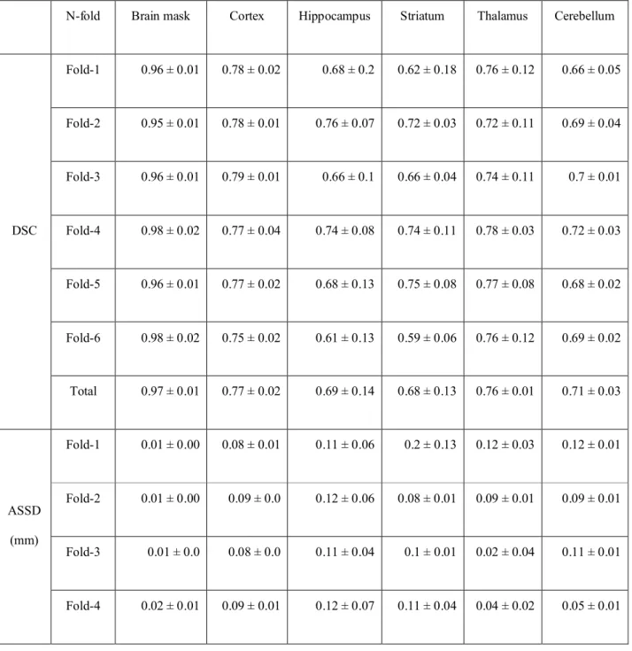
In Table 1, VOIDLand VOIiGTof 36 mice in target VOIs (cortex, hippocampus, striatum, thalamus, and cerebellum) were evaluated by calculating the average of DSC, ASSD, SEN, SPE, and PPV. Respectively, the DSC for each target VOI was 0.75, 0.68, 0.69, 0.74, 0.80, the ASSD was 0.04 mm, 0.05 mm, 0.13 mm, 0.04 mm, and 0.03 mm, SEN was 0.80, 0.69, 0.65, 0.79, and 0.74, SPE was 1.0, 1.0, 1.0, 1.0, and 0.99, and PPV was 0.78, 0.74, 0.80, 0.74, and 0.89, indicating that our DL model generated target VOIs well.
In Figure 4, the mean counts obtained by VOIDL, VOIiGT, and VOIGTwere significantly (p < 0.001) correlated with one another in all target VOIs. In addition, we conducted a correlation analysis between each SUVR obtained using VOIDL, VOIiGT, and VOIGTin all target VOIs (Figure 5). For SUVR analysis, cerebellum was used as a reference region, that is, mean counts of target regions were normalized by that of cerebellum. In all target VOIs, SUVR values obtained through VOIDL, VOIiGT, and VOIGTwere significantly (p < 0.001) correlated with one another. As shown in Figure 5b, in the hippocampus and thalamus, the mean SUVR obtained by VOIGTin template space and the VOIDLin individual space were almost identical, whereas in the cortex and striatum, the mean SUVR obtained by VOIGTwere slightly
underestimated compared to the mean SUVR obtained by VOIDL.
In Figure7-8, the trend of data was analyzed through the Bland-Altman plots. Mean counts and SUVR values obtained by VOIDLshowed mild overestimation with respect to that obtained by VOIiGTin cortex and striatum. This is not considered to be a significant difference in terms of the range of mean counts values. On the other hand, in hippocampus and thalamus, both mean counts and SUVR values obtained by three methods showed almost same trend.
Figure 3
Figure 4
Figure 5
Figure 6
Figure 7
3.3 Deep CNN for automatic generation of iVOI template in individual brain space using only PET images.
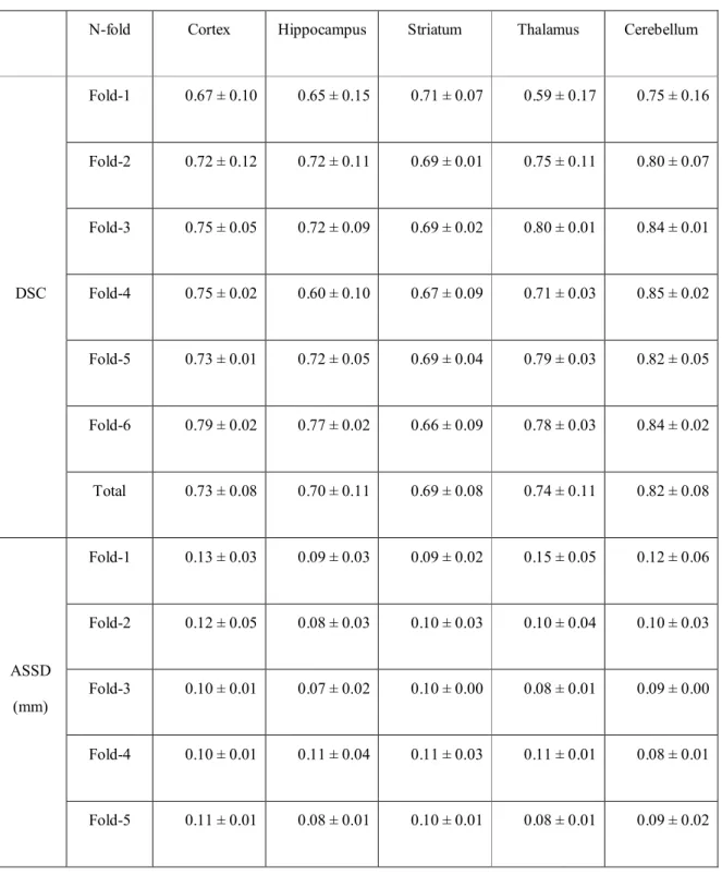
Figure 8a shows the axial slice of VOIDL(blue contour) and VOIiGT(red contour) in target VOIs (cortex, hippocampus, striatum, thalamus, and cerebellum) overlaid on the corresponding input images (i.e., skull-stripped PET images). In this case, we used PET images as a DL model input as in Figure 8a, we supplemented Figure 8b to see if there is any flaws in our method as compared with more anatomically-oriented image (i.e., corresponding T2-weighted MR). In visual assessment, high concordant between VOIDL and VOIiGTwas shown in all target VOIs. In Table 2, VOIDLand VOIiGTof 36 mice in target VOIs were evaluated by calculating the average of DSC, ASSD, SEN, SPE, and PPV. Respectively, the DSC for each target VOI was 0.73, 0.70, 0.69, 0.74, and 0.82, the ASSD was 0.05 mm, 0.04 mm, 0.04 mm, 0.03 mm, and 0.02 mm, SEN was 0.71, 0.61, 0.59, 0.65, and 0.78, SPE was 1.0, 1.0, 1.0, 1.0, and 1.0, and PPV was 0.79, 0.86, 0.86, 0.90, and 0.88, indicating that our DL model generated target VOIs well.
In Figure 9, the scatter plot and correlation analysis results of mean counts obtained by three methods (i.e., VOIDL, VOIiGT, and VOIGT) showed significantly correlated (p < 0.001, concordance correlation coefficient (CCC > 0.99) in all target VOIs. In addition, in Figure 10, the SUVR analysis showed concordant results between all VOI methods, forming line of identity and significant correlation (p < 0.001, CCC > 0.95).
In Figure11-13, the trend of data was analyzed through the Bland-Altman plots. Mean counts obtained by VOIDLshowed mild overestimation with respect to that obtained by VOIiGTand VOIGTin cortex, striatum and cerebellum. This is not considered to be a significant difference in terms of the range of mean counts values due to the nature of low-resolution PET images. On the other hand, in hippocampus and thalamus, both mean counts and SUVR values obtained by three methods showed almost same trend.
Figure 8
Figure 9
Figure 10
Figure 11
Figure 12
4 Discussions and Conclusion
SN of individual brain PET images onto standard anatomical spaces is required for objective statistical evaluation [6]. To do this, MR-based SN has been preferred to project individual brain PET and/or MR images into a template space [36, 37] because MRI is independent of changes in uptake patterns due to disease-induced abnormal uptake patterns in PET images and is advantageous in terms of anatomical precision. However, there is a limitation in that MR images corresponding to PET images cannot always be expected in the real world of clinical/preclinical practices. In addition, several steps of the preprocessing were semiautomatic, which causes time-consuming problems and inter- and intra-rater problem. In human brain studies, many neuroimaging analysis tools including SPM, FMRIB Software Library (FSL – [38, 39]) and Elastix [40, 41] have been widely used to perform SN. However, there are limitations in the use of these tools in mouse brain research due to various differences between human and mouse brains, such as the scale, shape, and image contrast (including distribution of gray matter).
A precise SN method through DL has also been devised and has recently attracted considerable attention.
However, despite the use of a complicated networks, the method still has difficulty in performing complete SN from affine transformation to nonlinear transformation [20] and an additional spatial normalization process is required to generate a pseudoPET template [31] or a method of generating MR from a PET image [23]. In addition, many studies have considered the use of iSN for PET quantitative analysis [25-27]. Representatively, iVOIs were defined using the iSN of the Brodmann area or callosal template VOIs as the seed points for diffusion tensor tractography [42, 43]. Although attenuation correction (AC) can be conducted directly using CT data in conventional PET/CT, it is difficult to conduct AC in PET/MR. To resolve this issue, several studies have employed template-based AC [44-47]. In particular, Sekine et al. (2016) [45] projected an atlas-based pseudo-CT to a patient-specific PET/MR space using iSN methods, which generated a single-head atlas from multiple CT head images. Inspired by this, we generated an iVOI template to reformulate the complicated and difficult-to-implement SN problem into a relatively simpler problem of VOI
segmentation for PET quantification. Overall, we have devised a unified CNN framework for brain mask generation in order to conduct skull-stripping and generate an iVOI template in individual space to perform precise PET quantification without any additional efforts of skull-stripping and SN. Additionally, iVOI generation deep learning was performed only with PET images, considering the actual clinical/preclinical environments where it is difficult to obtain MR images corresponding to PET in all cases.
With regard to DL for brain parenchyma segmentation, as shown in Figure 2, manually-traced brain mask contours (red) and DL-based contours (blue) were almost identical in visual assessment. Moreover, DSC reached 0.97, ASSD was less than 0.01 mm, and SEN and PPV were higher than 0.92 0.99 (Table 1) in comparison between these two masks, confirming good agreement from a quantitative perspective as well. With regard to DL for iVOI template segmentation, mean counts and SUVR values obtained by VOIiGTand VOIDLwere significantly (p < 0.001) correlated with each other in all target VOIs (cortex, hippocampus, striatum, thalamus, and cerebellum)(Figure3a, 4a). In addition, each of the mean counts and SUVR values obtained by template-based VOI (i.e. VOIGT) and individual space VOI (i.e.
VOIDL, VOIiGT) showed a significant (p < 0.001) correlation between each VOI methods (Figure 3b, 3c, Figure 4b, 4c).
However, the mean counts and SUVR values obtained by VOIGTtended to be slightly underestimated compared to that obtained by VOIiGTand VOIDLin hippocampus and striatum. Consequently, the % change of SUVR values in the target VOI showed the same tendency in each of the three methods. Considering the real world clinical/preclinical environment in which it is difficult to obtain MR images corresponding to PET in all cases, we established a model that generates iVOI only with PET images by varying inputs (i.e., skull-stripped PET images) in the same model as the previous iVOI generation model. In summary, we devise an unified deep CNN-based model that uses MR to generate brain masks for skull-stripping and iVOIs, as well as an iVOI-generated deep CNN-based model using PET images alone, as a novel method of PET quantitative evaluation in an individual SN-free space, avoiding variation between intra- and inter-rater that can occur in the preprocessing process. In addition, we showed a comparable level of segmentation performance using lighter neural network structures (i.e., CNNs with fewer training parameters—fewer channels and simple convolutional blocks) as compared with conventional mouse brain studies [10, 14]. Furthermore, our DL-based iVOI method has reformulated the PET SN problem for precise PET quantification, which remains challenging despite using a complicate network that requires a considerable parameter estimation [20, 23, 30], with an easy-to-handle image generation method for target VOIs using inversely normalized template VOIs.
This study involves several limitations. First, we only had small number of data, consisting of 18 mice.
Although the data was inflated by using consecutive axial slices of T2-weighted MR as multi-channels input of the deep CNN and by using data augmentation, this was not sufficient. In this light, cross-validation was performed by dividing the data into only train and test sets, but it is more desirable to train and evaluate the model with dividing the dataset into training/test/validation sets to prevent the deep learning model from overfitting to a specific dataset, in turn, to establish the model of greater generalization ability [46, 47]. Second, because this study was carried out with only in-house mice, there is a possibility that the trained model may be specialized to our data. Therefore, as in study by De Feo el al. (2021)
[14], model validation should be warranted with more data and various type of mice in the near future. In addition, mouse models do not have much variability in brain anatomy between individuals, so the deep learning model proposed in this study may have been easier than in the human brain. Moreover mouse used in this study consists of only mouse suffering from AD – the anatomical variability between mice may be minimal. Therefore, in future studies, the same experiment should be conducted using study population of both normal mouse and abnormal mouse to demonstrate the generalization ability of our devised deep learning model.
5 Conclusion
We proposed a unified deep CNN-based model that can generate mouse brain parenchyma masks and iVOI templates in individual brain space without any efforts or skull-stripping and SN. Through qualitative and quantitative evaluations, our devised model has shown highly concordant quantification of regional glucose metabolism (i.e., mean of radioactivity counts in each VOI) forming line of identity between ground-truth (conventional template) methods-based mean counts/SUVR and our devised DL-based mean counts/SUVR (Figures 4-5 and Figure 10-11). These results showed that the proposed approach may comprise a new method for PET image analysis by reformulating the SN problem, which has been difficult to implement despite of recent advances in DL techniques, into a segmentation problem using iVOI template generation in an individual brain space. Moreover, we implemented only PET-based iVOI generation to better cope with real world PET data without corresponding MRIs. In conclusion, this study established a new method based on deep CNNs to generate individual brain space VOI with neither SN nor MR.
6 Reference
1. Som P, Atkins HL, Bandoypadhyay D, Fowler JS, MacGregor RR, Matsui K, et al. A fluorinated glucose analog, 2-fluoro-2-deoxy-D-glucose (F-18): nontoxic tracer for rapid tumor detection. J Nucl Med. 1980;21:670-5.
2. Bascuñana P, Thackeray JT, Bankstahl M, Bengel FM, Bankstahl JP. Anesthesia and Preconditioning Induced Changes in Mouse Brain [(18)F] FDG Uptake and Kinetics. Mol Imaging Biol. 2019;21:1089-96.
3. Ma D, Cardoso MJ, Modat M, Powell N, Wells J, Holmes H, et al. Automatic structural parcellation of mouse brain MRI using multi-atlas label fusion. PLoS One. 2014;9:e86576.
4. Acosta-Cabronero J, Williams GB, Pereira JM, Pengas G, Nestor PJ. The impact of skull-stripping and radio- frequency bias correction on grey-matter segmentation for voxel-based morphometry. Neuroimage. 2008;39:1654- 65.
5. Fein G, Landman B, Tran H, Barakos J, Moon K, Di Sclafani V, et al. Statistical parametric mapping of brain morphology: sensitivity is dramatically increased by using brain-extracted images as inputs. Neuroimage.
2006;30:1187-95.
6. Feo R, Giove F. Towards an efficient segmentation of small rodents brain: A short critical review. J Neurosci Methods. 2019;323:82-9.
7. Nie J, Shen D. Automated segmentation of mouse brain images using multi-atlas multi-ROI deformation and label fusion. Neuroinformatics. 2013;11:35-45.
8. Yasuno F, Hasnine AH, Suhara T, Ichimiya T, Sudo Y, Inoue M, et al. Template-based method for multiple volumes of interest of human brain PET images. Neuroimage. 2002;16:577-86.
9. Kuhn FP, Warnock GI, Burger C, Ledermann K, Martin-Soelch C, Buck A. Comparison of PET template-based and MRI-based image processing in the quantitative analysis of C11-raclopride PET. EJNMMI Res. 2014;4:7.
10. Hsu LM, Wang S, Ranadive P, Ban W, Chao TH, Song S, et al. Automatic Skull Stripping of Rat and Mouse Brain MRI Data Using U-Net. Front Neurosci. 2020;14:568614.
11. Chou N, Wu J, Bai Bingren J, Qiu A, Chuang KH. Robust automatic rodent brain extraction using 3-D pulse- coupled neural networks (PCNN). IEEE Trans Image Process. 2011;20:2554-64.
12. Oguz I, Zhang H, Rumple A, Sonka M. RATS: Rapid Automatic Tissue Segmentation in rodent brain MRI. J Neurosci Methods. 2014;221:175-82.
13. Liu Y, Unsal HS, Tao Y, Zhang N. Automatic Brain Extraction for Rodent MRI Images. Neuroinformatics.
2020;18:395-406.
14. De Feo R, Shatillo A, Sierra A, Valverde JM, Gröhn O, Giove F, et al. Automated joint skull-stripping and segmentation with Multi-Task U-Net in large mouse brain MRI databases. Neuroimage. 2021;229:117734.
15. Jorge Cardoso M, Leung K, Modat M, Keihaninejad S, Cash D, Barnes J, et al. STEPS: Similarity and Truth Estimation for Propagated Segmentations and its application to hippocampal segmentation and brain parcelation.
Med Image Anal. 2013;17:671-84.
16. Ma D, Cardoso MJ, Modat M, Powell N, Wells J, Holmes H, et al. Automatic structural parcellation of mouse brain MRI using multi-atlas label fusion. PLoS One. 2014;9:e86576.
17. Kang SK, Seo S, Shin SA, Byun MS, Lee DY, Kim YK, et al. Adaptive template generation for amyloid PET using a deep learning approach. Hum Brain Mapp. 2018;39:3769-78.
18. Jaderberg M, Simonyan K, Zisserman A. Spatial transformer networks. Advances in neural information processing systems. 2015;28.
19. Detlefsen NS, Freifeld O, Hauberg S. Deep Diffeomorphic Transformer Networks. 2018 IEEE/CVF Conference on Computer Vision and Pattern Recognition; 2018. p. 4403-12.
20. Alvén J, Heurling K, Smith R, Strandberg O, Schöll M, Hansson O, et al. A Deep Learning Approach to MR-less Spatial Normalization for Tau PET Images. International Conference on Medical Image Computing and
Computer-Assisted Intervention: Springer; 2019. p. 355-63.
21. Delzescaux T, Lebenberg J, Raguet H, Hantraye P, Souedet N, Gregoire MC. Segmentation of small animal PET/CT mouse brain scans using an MRI-based 3D digital atlas. Annu Int Conf IEEE Eng Med Biol Soc.
2010;2010:3097-100.
22. Bai J, Trinh TL, Chuang KH, Qiu A. Atlas-based automatic mouse brain image segmentation revisited: model complexity vs. image registration. Magn Reson Imaging. 2012;30:789-98.
23. Choi H, Lee DS. Generation of Structural MR Images from Amyloid PET: Application to MR-Less Quantification. J Nucl Med. 2018;59:1111-7.
24. Ashburner J, Andersson JL, Friston KJ. Image registration using a symmetric prior--in three dimensions. Hum Brain Mapp. 2000;9:212-25.
25. Kim JS, Lee JS, Park MH, Kim KM, Oh SH, Cheon GJ, et al. Feasibility of template-guided attenuation correction in cat brain PET imaging. Mol Imaging Biol. 2010;12:250-8.
26. Kim JS, Cho H, Choi JY, Lee SH, Ryu YH, Lyoo CH, et al. Feasibility of Computed Tomography-Guided Methods for Spatial Normalization of Dopamine Transporter Positron Emission Tomography Image. PLoS One.
2015;10:e0132585.
27. Cho H, Kim JS, Choi JY, Ryu YH, Lyoo CH. A computed tomography-based spatial normalization for the analysis of [18F] fluorodeoxyglucose positron emission tomography of the brain. Korean J Radiol. 2014;15:862- 70.
28. Lehmann M, Douiri A, Kim LG, Modat M, Chan D, Ourselin S, et al. Atrophy patterns in Alzheimer's disease and semantic dementia: a comparison of FreeSurfer and manual volumetric measurements. Neuroimage.
2010;49:2264-74.
29. Palumbo L, Bosco P, Fantacci ME, Ferrari E, Oliva P, Spera G, et al. Evaluation of the intra- and inter-method agreement of brain MRI segmentation software packages: A comparison between SPM12 and FreeSurfer v6.0.
Phys Med. 2019;64:261-72.
30. Ashburner J, Friston KJ. Nonlinear spatial normalization using basis functions. Hum Brain Mapp. 1999;7:254-66.
31. Han S, Oh JS, Lee JJ. Diagnostic performance of deep learning models for detecting bone metastasis on whole- body bone scan in prostate cancer. Eur J Nucl Med Mol Imaging. 2022;49:585-95.
32. Jimenez-Carretero D, Bermejo-Peláez D, Nardelli P, Fraga P, Fraile E, San José Estépar R, et al. A graph-cut approach for pulmonary artery-vein segmentation in noncontrast CT images. Med Image Anal. 2019;52:144-59.
33. Kim H, Jung J, Kim J, Cho B, Kwak J, Jang JY, et al. Abdominal multi-organ auto-segmentation using 3D-patch- based deep convolutional neural network. Sci Rep. 2020;10:6204.
34. Hu YC, Mageras G, Grossberg M. Multi-class medical image segmentation using one-vs-rest graph cuts and majority voting. J Med Imaging (Bellingham). 2021;8:034003.
35. Gispert JD, Pascau J, Reig S, Martínez-Lázaro R, Molina V, García-Barreno P, et al. Influence of the
normalization template on the outcome of statistical parametric mapping of PET scans. Neuroimage. 2003;19:601- 12.
36. Woolrich MW, Jbabdi S, Patenaude B, Chappell M, Makni S, Behrens T, et al. Bayesian analysis of neuroimaging data in FSL. Neuroimage. 2009;45:S173-86.
37. Jenkinson M, Beckmann CF, Behrens TE, Woolrich MW, Smith SM. FSL. Neuroimage. 2012;62:782-90.
38. Klein S, Staring M, Murphy K, Viergever MA, Pluim JP. elastix: a toolbox for intensity-based medical image registration. IEEE Trans Med Imaging. 2010;29:196-205.
39. Shamonin DP, Bron EE, Lelieveldt BP, Smits M, Klein S, Staring M. Fast parallel image registration on CPU and GPU for diagnostic classification of Alzheimer's disease. Front Neuroinform. 2013;7:50.
40. Oh JS, Song IC, Lee JS, Kang H, Park KS, Kang E, et al. Tractography-guided statistics (TGIS) in diffusion tensor imaging for the detection of gender difference of fiber integrity in the midsagittal and parasagittal corpora callosa.
Neuroimage. 2007;36:606-16.
41. Oh JS, Kubicki M, Rosenberger G, Bouix S, Levitt JJ, McCarley RW, et al. Thalamo-frontal white matter alterations in chronic schizophrenia: a quantitative diffusion tractography study. Hum Brain Mapp. 2009;30:3812- 25.
42. Hofmann M, Pichler B, Schölkopf B, Beyer T. Towards quantitative PET/MRI: a review of MR-based attenuation correction techniques. Eur J Nucl Med Mol Imaging. 2009;36 Suppl 1:S93-104.
43. Hofmann M, Bezrukov I, Mantlik F, Aschoff P, Steinke F, Beyer T, et al. MRI-based attenuation correction for whole-body PET/MRI: quantitative evaluation of segmentation- and atlas-based methods. J Nucl Med.
2011;52:1392-9.
44. Wollenweber SD, Ambwani S, Delso G, Lonn AHR, Mullick R, Wiesinger F, et al. Evaluation of an Atlas-Based PET Head Attenuation Correction Using PET/CT & MR Patient Data. IEEE Transactions on Nuclear Science. 2013;60:3383-90.
45. Sekine T, Buck A, Delso G, Ter Voert EE, Huellner M, Veit-Haibach P, et al. Evaluation of Atlas-Based Attenuation Correction for Integrated PET/MR in Human Brain: Application of a Head Atlas and Comparison to True CT-Based Attenuation Correction. J Nucl Med. 2016;57:215-20.
46. Han S, Oh JS, Lee JJ. Diagnostic performance of deep learning models for detecting bone metastasis on whole- body bone scan in prostate cancer. Eur J Nucl Med Mol Imaging. 2022;49:585-95.
47. Han S, Oh JS, Kim Y-i, Seo SY, Lee GD, Park M-J, et al. Fully Automatic Quantitative Measurement of 18F- FDG PET/CT in Thymic Epithelial Tumors Using a Convolutional Neural Network. Clinical Nuclear Medicine. in press.
7 Korean Abstract
목적 생쥐의 뇌 양전자 방출 단층 촬영(Brain PET)의 정확한 정량분석을 위해서는 정밀한 두개골 제거 및 뇌 관심 영역 분할이 필요하다. 최근 딥러닝의 눈부신 발전으로 많은 의료영상처리의 문제들이 딥러닝으로 해결되어 왔으나, 공간 정규화를 딥러닝으로 해결하는 것은 아직까지 온전히 해결되기 어려운 문제로 남아있다. 또한 일반적인 전임상/임상 환경에서 PET 영상과 대응되는 자기공명영상 및 관련 관심영역 표준판이 항상 구비되어 있기는 어렵다. 따라서 본 연구에서는 이러한 문제를 해결하기 위해 수동으로 구획화 한 뇌 실질 마스크와 역 공간정규화에 의해 개별 뇌에 정의된 특정 관심 영역(피질, 해마, 선조체, 시상, 소뇌)을 레이블로 활용하여 훈련시킨 심층 신경망을 개발하였다. 나아가 이와 유사한 방법으로 자기공명영상 없이 PET 영상만을 입력으로 하여서도 동작하는 딥러닝 기반 관심영역 구획화를 구현하였다.
방법 본 연구에서는 알츠하이머병(Alzheimer’s disease)의 돌연변이 아밀로이드 전구체 단백질/프레세닐린-1 생쥐 모델을 사용하였다. 18 마리의 생쥐에 대하여 인간 면역글로빈 또는 항체
기반치료제를 투여하기 전(9 개월령)/후(10 개월령)로 두 번의 T2 강조 자기공명영상 영상과18F-FDG PET 영상을 촬영하였다. 딥러닝 훈련을 위해서 앞서 기술한 수동으로 생성한 뇌 마스크와 역 공간정규화 기반의 표적 관심영역이 레이블로 사용하였다. 모델 성능 평가를 위해 딥러닝 훈련에 사용된 레이블(즉, 역
공간정규화 표준 관심영역)과 딥러닝에 의해 생성된 관심부피영역 사이의 Dice similarity coefficient (DSC), average symmetric surface distance (ASSD), sensitivity (SEN), and positive predictive value (PPV) 를 평가하고 각 마스크(레이블 관심부피영역, 딥러닝 생성 관심부피영역) 및 표준판 공간상의 레이블
관심부피영역을 사용하여 평균 count 와 표준섭취계수율의 상관 관계를 비교하였다.
결과 본 연구에서 우리가 제안한 심층 합성곱 신경망 기반 방법은 자기공명영상을 사용하여 뇌 실질 마스크와 표적관심영역(즉, 피질, 해마, 선조체, 시상, 소뇌)을 성공적으로 생성했을 뿐만 아니라, 자기공명영상 없이 PET 이미지만으로도 표적 관심영역을 성공적으로 생성 가능함을 육안평가를 통하여 확인하였다. 또한 모든 표적관심영역에서 얻은 평균 count 와 표준섭취계수율은 자기공명영상을 사용한 방법과 PET 만을 사용한 각각의 방법 모두에서 레이블 관심영역에서 구한 값과 유의미한
상관관계(Concordant correlation coefficient > 0.97, P<0.001)를 나타내었다.
결론 본 연구에서는 두개골 제거 및 공간 정규화를 위해 별도의 큰 노력 없이 개별 뇌 공간에서 생쥐 뇌 실질 마스크와 역 공간정규화 기반 관심영역을 생성할 수 있는 통합 심층 합성곱 신경망 기반 모델을 제안함은 물론, 자기공명영상 없이 PET 영상 만으로도 이와 비교 가능한 성능을 보일 수 있는 심층 신경망 기반 모델을 제안하였다. 본 연구에서는 육안적 정성평가뿐 아니라 정량적 평가 (딥러닝 생성 표적관심영역과 레이블 표적관심영역간의 평균 count 및 표준섭취계수율의 비교)를 통해 그 값이 일치하는 것을 확인하였다.
결론적으로, 본 연구에서는 공간정규화나 수동 뇌 실질마스크 생성이 필요 없는 방식으로 자기공명영상 표준판 기반 관심영역을 기반으로 개별 뇌 표적관심영역을 생성함으로써, PET 영상 정량화를 위한 관심부피영역 구획화가 가능토록 하는 새로운 딥러닝 기반 방법을 확립하였다.
8 Figure Legends
Figure 1.Schematic diagram of our devised deep CNN model. (A) We conducted 6-fold cross-validation for training and test set separation. (B) Brain parenchymal mask generation deep CNN and inversely-normalized volumes-of-interest (iVOIs) in individual brain space generation deep CNN. For model training, T2-weighted magnetic resonance (T2 MR) imaging was used as an input and manually-traced brain mask was used as a label. Using the brain mask generated by the aforementioned model, skull-stripping of T2 MR was conducted and used as the model input to generate target VOIs (i.e., cortex, hippocampus, striatum, thalamus, and cerebellum). As the label for the model, iVOI template in individual space was used. (C) Deep CNN (i.e., U-Net) structure used in this study. The light blue box represents a 3 × 3
convolution and a leaky ReLU followed by max pooling, expressed in gray boxes. The orange and yellow boxes denote the 2 × 2 de-convolution and concatenation operations to increase the accuracy of localization. The dash arrow
represents the copying skip connections. The dash arrow represents the copying skip connections.
Abbreviation: deep convolutional neural network (deep CNN)
Figure 2.Comparison of mouse brain parenchyma mask contours between manually-traced brain mask (red contour) and deep CNN-predicted brain mask (blue contour) in three cases. The left shows the axial plane, the middle the coronal plane, and the right shows the sagittal plane.
Abbreviation: deep convolutional neural network (deep CNN)
Figure 3.Segmentation comparison of target VOIs (i.e., cortex, hippocampus, striatum, thalamus, cerebellum) in transaxial plane of three mice. The red contour represents deep learning label masks which are iVOI templates. The blue contour represents an iVOI template in an individual space generated by the proposed deep CNN.
Abbreviation: inversely-normalized VOI (iVOI); deep convolutional neural network (deep CNN)
Figure 4.Scatter plots between all mean counts (blue dot) obtained using VOIDL, VOIiGT, and VOIGTin all target VOIs from the first to the fifth row (cortex, hippocampus, striatum, thalamus, and cerebellum, respectively). CCC represents a measure of reliability based on covariation and correspondence. The line of identity (dashed line) is depicted as a reference line. (A) Correlation analysis between each mean count obtained using VOIDLand VOIiGT. (B) Correlation analysis between each mean count obtained using VOIDLand VOIGT. (C) Correlation analysis between each mean count obtained using VOIiGTand VOIGT.
Abbreviation: deep-learning generated-VOI (VOIDL); deep learning (inverse-normalized ground-truth) label VOI (VOIiGT); template-based ground-truth VOI (VOIGT); concordance correlation coefficient (CCC)
Figure 5.Scatter plots between all SUVR values (blue dot) obtained using VOIDL, VOIiGT, and VOIGTin all target VOIs from the first to the fourth rows (cortex, hippocampus, striatum, and thalamus, respectively). CCC represents a measure of reliability based on covariation and correspondence. The line of identity (dashed line) is depicted as a reference line.
(A) Correlation analysis between SUVR values obtained using VOIDLand VOIiGT. (B) Correlation analysis between SUVR values obtained using VOIDLand VOIGT. (C) Correlation analysis between SUVR values obtained using VOIiGT
and VOIGT.
Abbreviation: deep learning generated VOI (VOIDL); deep learning label VOI (VOIiGT); template-based VOI (VOIGT);
concordance correlation coefficient (CCC)
Figure 6.Bland-Altman plots are depicted to show the difference between all mean counts of radioactivity counts
obtained using VOIDL, VOIiGT, and VOIGTin all target VOIs from the first to the fifth row (cortex, hippocampus, striatum, thalamus, and cerebellum, respectively). The X-axis is the mean value of the two methods. The Y-axis represents the difference between two methods. Red line represents mean of the differences between the two results. The black dashed line represents 95% confidence interval. (A) Bland-Altman plot between each radioactivity counts obtained using VOIDL
and VOIiGT. (B) Bland-Altman plot between each radioactivity counts obtained using VOIDLand VOIGT. (C) Bland- Altman plot between each radioactivity counts obtained using VOIiGTand VOIGT.
Abbreviation: deep learning generated VOI (VOIDL); deep learning label VOI (VOIiGT); template-based VOI (VOIGT)
Figure 7.Bland-Altman plots are depicted to show the difference between all SUVR values obtained using VOIDL, VOIiGT, and VOIGTin all target VOIs from the first to the forth row (cortex, hippocampus, striatum, and thalamus, respectively). The X-axis is the mean value of the two methods. The Y-axis represents the difference between two methods. Red line represents mean of the differences between the two results. The black dashed line represents 95%
confidence interval. (A) Bland-Altman plot between each SUVR obtained using VOIDLand VOIiGT. (B) Bland-Altman plot between each SUVR obtained using VOIDLand VOIGT. (C) Bland-Altman plot between each SUVR obtained using VOIiGTand VOIGT.
Abbreviation: deep learning generated VOI (VOIDL); deep learning label VOI (VOIiGT); template-based VOI (VOIGT)
Figure 8.Segmentation comparison of target VOIs (i.e., cortex, hippocampus, striatum, thalamus, and cerebellum) in transaxial views in three mice. The red contour depicts deep learning label masks which are iVOI templates. The blue contour is for an iVOI generated, which is also in the individual brain space, by our devised deep CNN. (A) The label mask contour and the iVOI generated mask contour were overlaid on the PET image. (B) The label mask contour and the iVOI generated mask contour were overlaid on the T2-weighted MR (T2 MR) image to see if there are any flaws in our method as compared with more anatomically-oriented image (i.e., corresponding T2 MR).
Abbreviation: inversely-normalized VOI (iVOI); deep convolutional neural network (deep CNN); T2-weighted MR (T2 MR)
Figure 9.Scatter plot between all mean counts of radioactivity counts (blue dot) obtained using VOIDL, VOIiGT, and VOIGTin all target VOIs are depicted from the first to the fifth row (cortex, hippocampus, striatum, thalamus, and cerebellum, respectively). CCC represents a measure of reliability based on covariation and correspondence. The line of identity (dashed line) is depicted as a reference line. (A) Scatter plot between each mean count obtained using VOIDLand VOIiGT. (B) Scatter plot between each mean count obtained using VOIDLand VOIGT. (C) Scatter plot between each mean count obtained using VOIiGTand VOIGT.
Abbreviation: deep-learning generated-VOI (VOIDL); deep learning (inverse-normalized ground-truth) label VOI (VOIiGT); template-based ground-truth VOI (VOIGT); concordance correlation coefficient (CCC)
Figure 10.Scatter plot between all SUVR values (blue dot) obtained using VOIDL, VOIiGT, and VOIGTin all target VOIs are depicted from the first to the forth rows (cortex, hippocampus, striatum, and thalamus, respectively). CCC represents a measure of reliability based on covariation and correspondence. The line of identity (dashed line) is depicted as a reference line. (A) Scatter plot between SUVRs obtained using VOIDLand VOIiGT. (B) Scatter plot between SUVRs obtained using VOIDLand VOIGT. (C) Scatter plot between each SUVRs obtained using VOIiGTand VOIGT.
Abbreviation: deep learning generated VOI (VOIDL); deep learning label VOI (VOIiGT); template-based VOI (VOIGT);
concordance correlation coefficient (CCC)
Figure 11.Bland-Altman plots are depicted to show the difference between all mean counts of radioactivity counts obtained using VOIDL, VOIiGT, and VOIGTin all target VOIs from the first to the fifth row (cortex, hippocampus, striatum, thalamus, and cerebellum, respectively). The X-axis is the mean value of the two methods. The Y-axis represents the
difference between two methods. Red line represents mean of the differences between the two results. The black dashed line represents 95% confidence interval. (A) Bland-Altman plot between each radioactivity counts obtained using VOIDL
and VOIiGT. (B) Bland-Altman plot between each radioactivity counts obtained using VOIDLand VOIGT. (C) Bland- Altman plot between each radioactivity counts obtained using VOIiGTand VOIGT.
Abbreviation: deep learning generated VOI (VOIDL); deep learning label VOI (VOIiGT); template-based VOI (VOIGT)
Figure 12.Bland-Altman plots are depicted to show the difference between all SUVR values obtained using VOIDL, VOIiGT, and VOIGTin all target VOIs from the first to the forth row (cortex, hippocampus, striatum, and thalamus, respectively). The X-axis is the mean value of the two methods. The Y-axis represents the difference between two methods. Red line represents mean of the differences between the two results. The black dashed line represents 95%
confidence interval. (A) Bland-Altman plot between each SUVR obtained using VOIDLand VOIiGT. (B) Bland-Altman plot between each SUVR obtained using VOIDLand VOIGT. (C) Bland-Altman plot between each SUVR obtained using VOIiGTand VOIGT.
Abbreviation: deep learning generated VOI (VOIDL); deep learning label VOI (VOIiGT); template-based VOI (VOIGT)
9 Tables
Table 1.Evaluation of our unified deep neural network using MR by the mean and standard deviation of Dice similarity coefficient (DSC), average symmetric surface distance (ASSD) (mm), sensitivity (SEN), and positive predictive value (PPV) between deep learning labels and deep learning-generated brain masks and inversely-normalized target VOIs (cortex, hippocampus, striatum, thalamus, and cerebellum) in 6-fold cross validation.
N-fold Brain mask Cortex Hippocampus Striatum Thalamus Cerebellum
DSC
Fold-1 0.96 ± 0.01 0.78 ± 0.02 0.68 ± 0.2 0.62 ± 0.18 0.76 ± 0.12 0.66 ± 0.05
Fold-2 0.95 ± 0.01 0.78 ± 0.01 0.76 ± 0.07 0.72 ± 0.03 0.72 ± 0.11 0.69 ± 0.04
Fold-3 0.96 ± 0.01 0.79 ± 0.01 0.66 ± 0.1 0.66 ± 0.04 0.74 ± 0.11 0.7 ± 0.01
Fold-4 0.98 ± 0.02 0.77 ± 0.04 0.74 ± 0.08 0.74 ± 0.11 0.78 ± 0.03 0.72 ± 0.03
Fold-5 0.96 ± 0.01 0.77 ± 0.02 0.68 ± 0.13 0.75 ± 0.08 0.77 ± 0.08 0.68 ± 0.02
Fold-6 0.98 ± 0.02 0.75 ± 0.02 0.61 ± 0.13 0.59 ± 0.06 0.76 ± 0.12 0.69 ± 0.02
Total 0.97 ± 0.01 0.77 ± 0.02 0.69 ± 0.14 0.68 ± 0.13 0.76 ± 0.01 0.71 ± 0.03
ASSD (mm)
Fold-1 0.01 ± 0.00 0.08 ± 0.01 0.11 ± 0.06 0.2 ± 0.13 0.12 ± 0.03 0.12 ± 0.01
Fold-2 0.01 ± 0.00 0.09 ± 0.0 0.12 ± 0.06 0.08 ± 0.01 0.09 ± 0.01 0.09 ± 0.01
Fold-3 0.01 ± 0.0 0.08 ± 0.0 0.11 ± 0.04 0.1 ± 0.01 0.02 ± 0.04 0.11 ± 0.01
Fold-4 0.02 ± 0.01 0.09 ± 0.01 0.12 ± 0.07 0.11 ± 0.04 0.04 ± 0.02 0.05 ± 0.01
Fold-5 0.01 ± 0.00 0.09 ± 0.01 0.12 ± 0.08 0.1 ± 0.02 0.12 ± 0.01 0.07 ± 0.01
Fold-6 0.01 ± 0.0 0.09 ± 0.0 0.16 ± 0.08 0.11 ± 0.02 0.22 ± 0.08 0.15 ± 0.02
Total 0.01 ± 0.00 0.17 ± 0.0 0.12 ± 0.07 0.12 ± 0.06 0.1 ± 0.00 0.01 ± 0.00
SEN
Fold-1 0.91 ± 0.02 0.76 ± 0.05 0.67 ± 0.29 0.6 ± 0.15 0.68 ± 0.02 0.61 ± 0.05
Fold-2 0.94 ± 0.02 0.81 ± 0.04 0.66 ± 0.11 0.6 ± 0.06 0.65 ± 0.05 0.64 ± 0.12
Fold-3 0.93 ± 0.02 0.77 ± 0.03 0.53 ± 0.19 0.65 ± 0.08 0.69 ± 0.05 0.71 ± 0.14
Fold-4 0.97 ± 0.02 0.73 ± 0.06 0.7 ± 0.15 0.65 ± 0.14 0.69 ± 0.01 0.75 ± 0.05
Fold-5 0.88 ± 0.04 0.78 ± 0.07 0.55 ± 0.22 0.56 ± 0.12 0.66 ± 0.12 0.68 ± 0.08
Fold-6 0.87 ± 0.01 0.72 ± 0.07 0.52 ± 0.25 0.58 ± 0.08 0.64 ± 0.02 0.72 ± 0.07
Total 0.92 ± 0.02 0.76 ± 0.06 0.61 ± 0.22 0.61 ± 0.16 0.67 ± 0.05 0.69 ± 0.09
SPE
Fold-1 1.0 ± 0.0 1.0 ± 0.0 1.0 ± 0.0 1.0 ± 0.0 0.99 ± 0.0 0.99 ± 0.0
Fold-2 1.0 ± 0.0 1.0 ± 0.0 1.0 ± 0.0 1.0 ± 0.0 0.99 ± 0.0 0.99 ± 0.00
Fold-3 1.0 ± 0.0 1.0 ± 0.0 1.0 ± 0.0 1.0 ± 0.0 0.99 ± 0.0 1.0 ± 0.0
Fold-4 1.0 ± 0.0 1.0 ± 0.0 1.0 ± 0.0 1.0 ± 0.0 1.0 ± 0.0 1.0 ± 0.0
Fold-5 1.0 ± 0.0 1.0 ± 0.0 1.0 ± 0.0 1.0 ± 0.0 1.0 ± 0.0 1.0 ± 0.0
Fold-6 1.0 ± 0.0 1.0 ± 0.0 1.0 ± 0.0 1.0 ± 0.0 1.0 ± 0.0 1.0 ± 0.0
Total 1.0 ± 0.0 1.0 ± 0.0 1.0 ± 0.0 1.0 ± 0.0 0.99 ± 0.0 0.99 ± 0.0
PPV
Fold-1 0.98 ± 0.01 0.8 ± 0.03 0.65 ± 0.14 0.88 ± 0.04 0.73 ± 0.01 0.68 ± 0.03
Fold-2 0.99 ± 0.01 0.76 ± 0.02 0.67 ± 0.06 0.81 ± 0.03 0.8 ± 0.06 0.78 ± 0.07
Fold-3 0.99 ± 0.0 0.8 ± 0.02 0.67 ± 0.09 0.82 ± 0.05 0.78 ± 0.03 0.71 ± 0.03
Fold-4 0.99 ± 0.0 0.81 ± 0.01 0.6 ± 0.03 0.8 ± 0.06 0.82 ± 0.03 0.65 ± 0.02
Fold-5 0.99 ± 0.01 0.76 ± 0.03 0.72 ± 0.11 0.8 ± 0.04 0.77 ± 0.03 0.74 ± 0.03
Fold-6 0.99 ± 0.0 0.8 ± 0.05 0.58 ± 0.07 0.76 ± 0.01 0.78 ± 0.02 0.68 ± 0.04
Total 0.99 ± 0.0 0.79 ± 0.04 0.65 ± 0.1 0.81 ± 0.06 0.78 ± 0.03 0.71 ± 0.01
Table 2.Performance metrics of our only-PET-based deep neural network assessed through the mean and standard deviation of Dice similarity coefficient (DSC), average symmetric surface distance (ASSD) (mm), sensitivity (SEN), and positive predictive value (PPV) between deep learning labels and deep learning-generated brain masks and inversely- normalized target VOIs (cortex, hippocampus, striatum, thalamus, and cerebellum) in 6-fold cross validation.
N-fold Cortex Hippocampus Striatum Thalamus Cerebellum
DSC
Fold-1 0.67 ± 0.10 0.65 ± 0.15 0.71 ± 0.07 0.59 ± 0.17 0.75 ± 0.16
Fold-2 0.72 ± 0.12 0.72 ± 0.11 0.69 ± 0.01 0.75 ± 0.11 0.80 ± 0.07
Fold-3 0.75 ± 0.05 0.72 ± 0.09 0.69 ± 0.02 0.80 ± 0.01 0.84 ± 0.01
Fold-4 0.75 ± 0.02 0.60 ± 0.10 0.67 ± 0.09 0.71 ± 0.03 0.85 ± 0.02
Fold-5 0.73 ± 0.01 0.72 ± 0.05 0.69 ± 0.04 0.79 ± 0.03 0.82 ± 0.05
Fold-6 0.79 ± 0.02 0.77 ± 0.02 0.66 ± 0.09 0.78 ± 0.03 0.84 ± 0.02
Total 0.73 ± 0.08 0.70 ± 0.11 0.69 ± 0.08 0.74 ± 0.11 0.82 ± 0.08
ASSD (mm)
Fold-1 0.13 ± 0.03 0.09 ± 0.03 0.09 ± 0.02 0.15 ± 0.05 0.12 ± 0.06
Fold-2 0.12 ± 0.05 0.08 ± 0.03 0.10 ± 0.03 0.10 ± 0.04 0.10 ± 0.03
Fold-3 0.10 ± 0.01 0.07 ± 0.02 0.10 ± 0.00 0.08 ± 0.01 0.09 ± 0.00
Fold-4 0.10 ± 0.01 0.11 ± 0.04 0.11 ± 0.03 0.11 ± 0.01 0.08 ± 0.01
Fold-5 0.11 ± 0.01 0.08 ± 0.01 0.10 ± 0.01 0.08 ± 0.01 0.09 ± 0.02