The convergenece of finite difference approximations for singular two-point boundary Value Problems

THE CONVERGENCE OF FINITE DIFFERENCE APPROXIMATIONS FOR SINGULAR

TWO-POINT BOUNDARY VALUE PROBLEMS H. Y. LEE, J. M. SEONG, AND J. Y. SHIN

ABSTRACT. We consider two finite difference approximations to a singular boundary value problem arising in the study of a nonlinear circular membrane under normal pressure. It is shown that the rates of convergence areO(h) andO(h2 ),respectively. An iterative scheme is introduced which converges to the solution of the finite difference equations. Finally the numerical experiments are given

1. Introduction

In the study of a nonlinear circular membrane under normal pressure [3,4], the following singular boundary value problem arises:

(1.1)

" 3 , 2

- y - -y - - =0, 0< x < 1,

X y2

y'(O) =0, y'(1)+^{(1 - v)y(1)} =0, 0 < v < 1,

where v, 0 < v < 1, is a constant. The existence of a unique positive solution of (1.1) has been discussed by [2,3,4,9]. Numerical solutions of this problem can be obtained by the iterative method [2] and nu- merical techniques [4] on the integral equation equivalent to (1.1). It is mentioned in [4] that because of singularity and the nonlinearity, diffi- culties are encountered if numerical solutions of (1.1) are attempted by finite difference methods. In [8], a finite difference method to a class of singular boundary value problem is introduced.

When the boundary condition at x = 1 is y(1) = A(> 0) instead. of y'(1)+(1-v)y(1) =0, the unique existence of a positive solution and a

Received March 28, 1998.

1991 Mathematics Subject Classification: 65L12, 65LlO.

Key words and phrases: A finite difference approximation, a singular boundary value problem, a rate of convergence.

numerical solution are studied by [2,3,4,7,8,9]. In [7], a finite difference approximation to (1.1)isintroduced whose rate of convergenceisO(h²)

and which may avoid the above difficulties stated in[4]. And the global error estimateO(h²) is better than one in [8].

Inthis paper, motivated by the method in [7], two finite difference approximations to (1.1), scheme I and scheme II, are considered. The rates of convergence areO(h)andO(h²), respectively and both meth- ods may avoid the difficulties stated in [4]. To obtain the solution of each finite difference equation, an iterative technique is introduced which converges monotonically to the solution of the finite difference equation. Insection 2, some preliminaries are given. In section 3, two finite difference approximations, scheme I and scheme II, are intro- duced, and an iterative techniqueis given which converges monotoni- cally to the solution of the finite difference equations. Insection 4, we prove analytically that the rates of convergence of the scheme I and the schemeII are O(h) and O(h²), respectively. The rates of convergence of schemeI and schemeII are verified numerically in section 5.

2. Preliminaries

To discuss the behavior of the solution of (1.1) at x = 0, we begin with the following lemma whose proofis·straightforward.

LEMMA 2.1. Let f ^E C[O,l] and f' ^E C(O,l]. If tim f'(x) exists,

x-tO+

then

f' (0) = tim f(x)- f(O) = tim f'(x),

+ x-tO+ X x-tO+

which implies that f'(x) contmuousatx =^O.

Itwas shown in[9]that there exists a unique solutionYEC2(0,1]n

Cl[0, 1] of (1.1). Thus the following lemma is obtained from Lemma 2.1 and the fact that

1 [X ²⁸³

Y'(x) = - x3lo y2(S) ds.

LEMMA 2.2 [7]. Let Y be a positive solutionof(1.1). Then (1) Y~(O) existsandY"(x) is continuousat x = O.

(3.1.1)

(2) Y+(3)(0)(= 0) existsand ^y(3)(x) is continuousatx = o.

(3) Y+(4)(0) existsand y(4)(x) is continuousat x = o.

REMARK. Lemma 2.2 implies thatifY isa positive solution of (1.1) thenY EC⁴[0, 1].

3. Finite difference approximations 3.1. Scheme I

LetN be a positive integer, h= ~, ^{Xi = i-h, i} = 0,1,2, _. -,N,and let Yi be the approximation ofY(Xi), i = 0, 1, 2, ... , N. Consider the following finite difference approximation (scheme I):

_ 8 .Y1 - Yo - ~ = 0

h² Y5 '

_ 4. Y2 - 2Y1+^{Yo _} ~ = 0

h² Y f '

Yi+1 - 2Yi+Yi-1 3 Yi+1 - Yi-1 2 -""2=0,

h² Xi 2h Yi

i = 2, 3, ... , N - 1, YN-1 - YN + (1 ) 0

- h -v YN = .

Let

8 -8 0 0

-4 8 -4 0 0

0 3h 3h

- 1 + - 2 - 1 - -

2X2 2X2

£1= 0

0 0 - 1+ 3h 2 -1- 3h

2XN-1 2XN-1

0 0 -1 1+ h(1-v)

y= (Yo, Yl, ... , YN-l, YN)t,

and

N1y-= (_2h² _ 2h² ••. _ 2h²

O)t

2 ' 2 ' , 2 ' ,

Yo Y1 YN-1

whereN₁yandyare column vectors. Now we have a nonlinear system (3.1.2)

where 0 isthe zero vector. To solve the nonlinear system (3.1.2), we use Newton's method. So, for m = 0, 1, 2, "', we have

(3.1.3) y(Tn+l) = y(Tn) _ (L1+N1'y(Tn»)^{-1 .} (L1y(Tn) +N 1y(Tn») ,

h N ,-. h di al . di [4h² 4h² 4h² 0]

were 1 YISt e agon matrIX, ag - 3i - 3 ,'" ' - 3 - - ' .

Yo Y1 YN-1

Therefore, from (3.1.3), we derive

and

(3.1.5)

L 1y(Tn+1)+_{N 1y(Tn+1)}

= N1y(Tn+1) _ ^{N1y(Tn) _} N 1'y(Tn) [y(Tn+1) _ y(Tn)]

= ~N1I/e(Tn) ( (yjTn+1) _ yJTn»)

2) ,

h N ^{1 / - ' h di} al . di [12h² 12h² 12h² ]

were 1 YISt e agon matrIX, ag - -4-" - -4-' .. " - -4--,0 ,

Yo Yl YN-l

and ejTn) is between yJTn+1) and yjTn).

THEOREM 3.1.1 [1].

(i) The M-matrix L₁ is an inverse positive matrix.

(ii) The matrix L₁+ ^N1'y is an inverse positive matrix for any

y>O.

Proof (i) Let D_i be the (i +1)-th leading principal minor of L_{1 .} Then we obtain

Do =

8,

(1

DN-l =

(1

2

(1

2

which imply that the M-matrix L₁ is an inverse positive matrix.

(ii) Since L₁ is an M-matrix and N{y is a nonnegative diagonal matrix for' anyy >0, L₁+N1'y is an inverse positive matrix. 0

LEMMA 3.1.1. Ifu satisfies L₁u +NIU 2:: °^{and 1}satisfies L₁1+

NIl::; 0, then

1 ::; u,

where

°

°

Proof. From the assumptions on u and 1, we have 0::; L1U+N1u - L₁1-NIl

= L1(U-1)+N₁(u-1)

=(L1+N₁'e)(u-1),

where ei lies between ^li and ^Ui. Since L1 +N1'e is inverse positive,

u -12:: 0, which completes the proof. 0

LEMMA 3.1.2. Ifu satisfies L₁u +N₁u 2:: 0, yCO) > 0, L_1y(O) +

N1Y(O) ::; 0, and {yCrn)} is given by (3.1.3) or (3.1.4), then

yCO) ::; y(1) ::;y(2) ::; ... ::;y(m) ::; •.. ::; u for m =0, 1, 2, where 0< Ui for i =0, 1, 2, ... , N.

Proof It is obvious from (3.1.3), (3.1.5) and Lemma 3.1.1. 0 Let

lex) = _[ (1 - v)2 ]i(x2 _ 2 - v) 4(2-v)2 1 - v ' li =^l(ih),i= 0,1,2,'" ,N, 1=(lo,It,l2,', IN)t,

where h = k. ^{Then it is} easy to show that 1 satisfies L11+N11 ::; O.

And let

( )_ [(1 - v)2].!( 2 3 - v)

U X - - 3 X - - -

16 1-v '

Ui =u(ih),i=0,1,2"" ,N,

U = (Uo,Ul,U2,', UN)t.

Then it is alsoeasy to show that u satisfiesL1u +N1U ~ O.

THEOREM 3.1.2. The system ofequations (3.1.2) has a unique pos- itive solution.

Proof The system of equations (3.1.2) has a positive solution from Lemma3.1.2 and the above remark. Suppose that y andw are positive solutions of the system of equations (3.1.2) and z = y - w. Then we have

So we obtain

where ei ^{is betweenYi and Wi. Since L}1+^N1/eis an inverse positive

matrix, Z = 0 and hencey = w. 0

3.2. Scheme 11

Using the same notationsas given in the beginnig of Section3.1, we consider the following finite difference approximation (scheme II):

_ 8. Y1 - Yo - ~ =0

h² Y5 '

_ 4. Y2 - 2Y1 +Yo _ _~ =0

h² YI'

(3.2.1) _ Yi+1 - 2Yi +Yi-1 _ _~ . Yi+1 - Yi-1 _ _~ - 0

h² Xi 2h Yt - ,

i =2, 3, ". , N - 1,

2YN-1-2YN 2 3 2

- +-(1-V)YN+-(1-v)YN--=O.

h² h XN YFv

Let _{L 2} be the same matrix as the matrix L1 in section 3.1 except the n-th row and let the n-th row ofL2 be0,0, ... ,0, -2,2+2h(1-v) +3h²(1-v). Let

and

N2Y-= (_^{2h2 _ 2h2 ••• _ 2h2 _ 2h2) t}

2' 2' , 2 ' 2 '

Yo Y1 YN-1 YN

where N2Y and y are column vectors. Now we have a nonlinear system (3.2.2)

where 0 isthe zero vector. So, for m = 0, 1, 2, "., we have

where N2'y ^is the diagonal matrix, diag[~2,

Yo Therefore; from (3.2.3), we derive

and

(3.2.5)

L2y(m+1)+N2y(m+l)

= N2y(m+l) _ N2y(m) _ N2'y(m) [y(m+l) _ y(m)]

=~N2,,{(m) ((y~m+l)^-

yjm)f) ,

h l\T , , - . h di al . d· [12h² 12h² 12h²]

w erelV'2 Ylst e agon matrIX_, Jag - - - ... - - -_{4 ' 4 ' , 4 '}

Yo Y1 YN

and {~m)^is betweeny~m+l) and y~m).

THEOREM 3.2.1 [1].

(i) The M-matrixL2 isan inverse positivematrix.

(ii) The matrix L2 +N₂'y is an inverse positive matrix for any

y> 0.

Proof. (i) Let D_i be the (i +1)-th leading principal minor of L_{2 •} Then we obtain

Do =

8,

(1

::2)

D N-^l =

(1

2

DN = ^{2h(1-v)+^3h2(1-vH·

(1

2

which imply that theM-matrixL₂ isan inverse positive matrix.

(ii) The proofis the same as that of Theorem 3.1.1. 0 LEMMA 3.2.1. Ifu satisfies L2U+^{N2U ;;:::}

°

N21SO, then

1S u,

where0 <^Ui and 0 < h fori =0, 1, 2, ... , N.

Proof. The proof is similar to that of Lemma 3.1.1. o

LEMMA 3.2.2. H u satisfies L₂u +N₂u ;;::: 0, yCO) > 0, L2yCO) +

N2yCO) So, and{yCm)} is given by (3.2.3) or (3.2.4), then

yCO) S yCl) S y(2) S ... S yCm) S ... S u, for m = 0, 1, 2, ... ,

l(x) = _[ (1-v)2 ]!(x2 _ 2 - v) 4(2 - v)2 1-v ' li=l(ih),i=0,1,2,'" ,N, 1= (lo,Lt,b, "IN)t,

where h = 1. Then it is easy to show that 1 satisfies L21+N21~ O.

Andlet

u(x) = -

[(1

=:) ,

Ui = u(ih),i= 0,1,2,·,N,

u = (UO,Ul,U2,'" ,UN)t.

T~enit is also easy to show that u satisfies L2U+^N2U 2:O.

THEOREM 3.2.3. The system of equations (3.2.2) has a unique pos- itive solution.

Proof The proof is similar to that of Theorem 3.1.3. o

4. The convergence of finite difference approximations 4.1. Scheme I

LEMMA 4.1.1 [5,7]. Let Q(Xi) = Qi and E(Xi) = E i be dis- crete functions defined on xo, Xl, X2, " . , X N. Assume that there exists an w >

°

Qi ~ -w< 0, i = 0, 1, 2, ... , N - 1.

Set C = max(~,¹~^v). At the grid points Xo, ^Xl, X2, XN define a difference operatorLq ^by

h El-Eo

(4.1.1) LIEo= 8· h₂ +QoEo, ( 1 2) L hE - 4. E^{2 -} 2EI+Eo Q E

4. . I I - h₂ + I 1,

(4.1.3)

(4.1.4) Then

Proof. Note that C ~ 1. IfmaxIEiIoccurs for i =N, then

IENI ~ ¹~vIL~ENI.

Suppose that maxIEil occurs for one ofi = 0, 1, 2,'" , N - 1. Then from the proof of Lemma 4.1 in (7), we have

4 h

o<~~_IIEjl ~_3_ ^{w .}O<~~_IILIEjl·_3_

Thus the proofiscompleted. o

THEOREM 4.1.1. Let Y(x) E C4[0,1) be an analytic solution of the boundary value problem (1.1). Let Yi, i = 0, 1, 2, ... , N, be numerical solutions ofLIy+NIy =0 and Ei =Y(Xi) - Yi be errors.

Then

where

M⁴ =sup

I

I

[O,l}

(4.1.5)

Proof. By the mean value theorem and Taylor theorem, we obtain

" ( ) 2

0=4Y Xo + 2

[Y(xo)}

=^8.Y(XI) - Y(xo) 2 _ y(4)(~ ^{) . h2}

h2 + [Y(xO))2 0 3'

whereXo < ~o< ^Xl. ForXl, we have

(4.1.6)

" ( ) 3 ' ( . ) . 2

0= Y ^{Xl + - .}Y ^{Xl + 2}

Xl (y(XI))

= 4Y"(XI)+3(ylI(~O) - y"(XI)) + [Y(:I))2

=4.y(X2) - 2Y~:I)+Y(xo) _ ~ ^[y(4)(1]O) +y(4)(1]I)]

+3y(4)(~2)'~I(~O-Xl)+ ² 2,

[y(Xl))

whereXi-1 <170 < Xi <171 < XH!, Xi-1 < eo < e2 < Xi < ea ^{< e1 <}

Xi+!, Xo <e4 < Xi . And for XN, we obtain 0=^Y/(XN) +(1-V)Y(XN)

(4.1.8) = Y(XN)-h^Y(XN-1) +(1 - ^V)Y(XN) + ~Y"(eo).

whereXN-1 <eo < XN. From (3.1.1), (4.1.1), and (4.1.5) we obtain

h El - Eo (4) h²

L1E_{O= 8·} h₂ +QoEo= Y (eo)· 3·

From (4.1.2) and (4.1.6), we get L^hE = 4. E2 - 2E¹+Eo Q E

1 1 h2 + 1 1

= ~2 ^{[y(4)(170)+y(4)(171)] -} 3y(4)(6)6(eo - Xl).

And, from (4.1.3) and (4.1.7), we have

Lhg EH 1 - 2Ei +E i - ¹ ~. E i+^{1 -} Ei-l Q.g

1 Z h2 +^Xi 2h + ^{Z Z}

=h² [2y(4)(€4)+ y(4)(€2)(€o _ Xi) +y(4)(€3) (€l - Xi)]

2 Xi Xi

+ ~: ^{[y(4)(1]0) +y(4)(1Jl)] , i =}2, 3, ... , N-1.

From (4.1.4) and (4.1.8)

where F(y) = 2₂, Qi = ^F'(J-Li) = - ~ ^{::; -w < 0, and J-Li lies}

y \d^4';Z\"

betweenY(Xi) andYi· Let M4 =^{sup - d4 •} Then we obtain

[0,1] X

h² ILhEol::; 3 M4'

h²

ILhE11 ::; 3 M4+3h²M4 ,

h²

ILhEil ::; 12M4+2h²M4 , i = 2, 3, ... , N-1 ILhENI ::; 2"h^M4.

Thus,by Lemma 4.1.1, we have

IEil ::; CM4h, for i =0, 1, 2, ... , N,

which completes the proof. 0

4.2. Scheme 11

LEMMA 4.2.1. -"et Q(Xi) =^{Qi, E(Xi)} =E i be discrete functions defined on Xo, Xl, X2, ... , XN. Assume that there exists anw >

°

such that

Qi ~ -w < 0, i = 0, 1, 2, ... , N.

SetC=max(~, 2(1~V)). At thegridpointsxo, Xl, X2, " ' , XN define a difference operatorL~ by

(4.2.1) L~Ei =L}Ei , ⁱ = 0, 1, 2, ... , N -1,

h 2EN - 1 - 2EN 2 3

(4.2.2) L 2EN ⁼ h 2 -;;,(1-v)EN - XN (l-v)EN+QNEN.

Then

IEil ~^{C· max [} ~ax IL~Ejl, hIL~ENI], ^{i =} 0, 1, 2, ... , N.

0'5.J'5.N-1

Proof. Note that C 2:: 1. IfmaxIEil occurs for ⁱ =N, then

h h

jENI ~ ^{2(1 _ v) IL2EN)'}

Suppose that maxIEiIoccurs for one ofi =0, 1, 2, ... , N - 1. Then sinceLqEi = L~Ei, i = 0, 1, 2,;" N - 1, the remaining part of the

proof is the same as that of Lemma 4.1.1. 0

Since Y(x) E C⁴[0,1] and Y(l) > 0, we may extend the positive solution of (1.1) to the interval [0,1+^8], for sufficiently smallD> 0.

So we have the following theorem whose proof is the same as that of Theorem 4.1.1.

THEOREM 4.2.1. Let Y(x) E C⁴[0,1+<5], be an analytic solution ofthe boundary value problem (1.1) for sufficiently small <5 > 0. Let Yi be numerical solutions of L 2y+N2Y = 0 and E i ⁼ Y(Xi) - Yi be errors, where^{i =} 0, 1, 2, .. , , N. Then

- 2

IEil ~ CM4h, where

- \d⁴

y\

M4= sup - -

[0,1+6] dx⁴ and C isa constant.

(4.2.3)

Proof. From (1.1), by the mean value theorem and Taylor theorem, we obtain

"( ) 3 ' ( ) 2

0=Y XN + - .^{Y XN} + ²

XN [Y(XN)]

= Y(XN+1) - 2Y(XN)+Y(XN-1) _ (1- V)~Y(XN)

h² XN

+ [Y(:N)]2 - ~: ^{[y(4)(17O)+y(4)(111)] ,}

where XN-1 <110 < XN <711 < XN+1. And we obtain (4.2.4)

Y(XN+l)~^Y(XN-1) +(1-V)Y(XN) - ~ [y(3)(~0)+y(3)(6)] = 0, where XN-1 < ~o < XN < 6 < XN+l. By substituting (4.2.4) into (4.2.3), we get

0= 2Y(XN-1~;^{2Y(XN) _} ~(1-^V)Y(XN)+~[2y(4)(~4)

(4.2.5) +y(4)(~2)(~0 ^{- XN)+}y(4)(6)(~1 ^{- XN)] + [Y(:N)]2}

_ h 2

[y(4)(110) +^y(4)(11t)] - (1-v)~Y(XN)'

24 XN

where XN < 6 <XN+l, XO < ~4 < XN. Therefore we have

h 2EN- 1 -2EN 2 3

L_2EN - -(1-_{v)EN -} - ( 1 -V)EN +_QNEN

h² h XN

= - ~ [2y(4)(~4)+y(4)(~2)(~0 ^{- XN)} +^y(4)(6)(6 - XN)]

h²

+ 24[y(4)(110)+y(4)(111)],

where F(y) = 2₂, Qi = F'(JLi) = - ⁴₃ ^::; -w < ^0, JLi lies between

y JLi

Y(Xi) and Yi. Since _L~Ei = L~Ei, i = 0, 1, 2, ., N - 1, we obtain from the proof of Theorem 4.1.1

I_{L2Ei ::;}^h I _CM-_4h²_{,i =} 0, 1, 2, ... , N -1

and from (4.2.5) we get

_ I

d4Y

where M4 = sup d 4 Ifor sufficiently small 8>0. Thus, by Lemma

[0,1+6) x 4.2.1, we have

- 2

IEil ~ CM₄h, for i = 0, 1, 2, ... , N,

which completes the proof. 0

5. Numerical experiments 5.1. Scheme I

The scheme I, proposed in section 3.1, has been implemented on an

mM pc.Inthe computation, we use

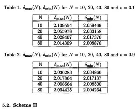
to stop the iteration when we solve the nonlinear system (3.1.2) by Newton's method (3.1.3) or (3.1.4). Intable 1, we report the values of 8_max{N) and 8min{N) for N =10, 20, 40, 80 andv =^{0.1, where}

andYN represents the solution of the nonlinear system (3.1.2) for the given N. And in table 2, the value of 8max{N) and 8_min{N) are given for N =10, 20, 40, 80 andv =0.9. From table 1 and table 2, we see numerically that Theorem 4.1.1 is valid.

Table 1. dmax(N), dmin(N) for N = 10, 20, 40, 80 andv= 0.1

N dmax(N) dmin(N)

10 2.109554 2.059469 20 2.055978 2.033158 40 2.028407 2.017376 80 2.014309 2.008876

Table 2. dmax(N), dmin(N) for N = 10, 20, 40, 80 and v= 0.9

N dmax(N) dmin(N)

10 2.036283 2.034866 20 2.017864 2.017137 40 2.008664 2.008500 80 2.004415 2.004234

5.2. Scheme 11

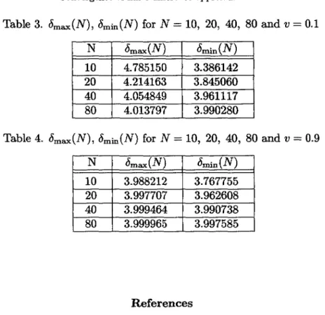
The scheme Il, proposed insection 3.2, has also been implemented on anmMPC.Inthe computation, we use

j=O,e~N_1Iy(k+1)(Xj)^{- y(k)(Xj)}

I

to stop the iteration when we solve the nonlinear system (3.2.2) by Newton's method (3.2.3) or (3.2.4). Intable 3 we report the values of dmax(N) and dmin(N) for N =10, 20, 40, 80 andv =^{0.1, where}

~ (N) _ IY2N(Xj) - YN(Xj)I

Qmax - max ,

j=O,l,···,N IY4N(Xj) - Y2N(Xj)I

dmin(N) = min IY2N(Xj) - YN(Xj)I

j=O,l,···,N IY4N(Xj) -Y2N(Xj)1

and YN represents the solution of the nonlinear system (3.2.2) for the givenN. Andin table 4 the value ofdmax(N) and dmin(N) are given for N = 10, 20, 40, 80 andv = 0.9. From table 3 and table 4, we see numerically that Theorem 4.2.1 isvalid.

Table 3. tSmax (N), tSmin (N) ^for N =10, 20, 40, 80 andv =0.1

N tSmax(N) tSmin(N)

10 4.785150 3.386142 20 4.214163 3.845060 40 4.054849 3.961117 80 4.013797 3.990280

Table 4. tSmax(N), tSmin(N) for N =10, 20, 40, 80 and v=^0.9

N tSmax(N) tSmin(N) 10 3.988212 3.767755 20 3.997707 3.962608 40 3.999464 3.990738 80 3.999965 3.997585

References

[1] A. Berman & R. J. Plemmons, Nonnegative Matrices in the Mathematical Sciences, SIAM, Philadelphia, 1994.

[2] E. Bohl, On two boundary value problems in nonlinear elasticity from a nu- merical viewpoint (R. Ansorge, W. Toring, 1-14, ed.), In: Lecture Notes in Mathematics No. 676, Springer, Berlin, 1974.

[3] A.J. Calligari& E. L. Reiss, Nonlinear boundary value problems for the circular membrane, Arch. Rat. Mech. Anal. 31 (1970),390-400.

[4] R. W. Dickey, The plane circular elastic surface under normal pressure, Arch.

Rat. Mech. Anal. 26 (1967), 219-236.

[5] D. Greenspan& V. Casulli, Numerical Analysis for Applied Mathematics, Sci- ence, and Engineering, Addison-Wesley Publishing Company, New York, 1988.

[6] B. Gustafsson, A numerical method for solving singular boundary value prob- lems, Numer. Math 21 (1973),328-344.

(7] H. Y. Lee, M. R. Ohm and J. Y. Shin, A finite difference approximation of a singular boundary value problem, Bull. Korean Math. Soc. (accepted).

[8] R. N. Sen & Md. B. Hossain, Finite difference methods for certain singular two-point boundary value problems, Journal of Computational and Applied Mathematics 70 (1996), 33-50.

[9] J. Y. Shin, A singular nonlinear boundary value problem in the nonlinear cir- cular membrane under normal pressure,J.Korean Math. Soc. 32 (1995), no. 4, 761-773.

H. Y. Lee, J. M. Seong Department of Mathematics Kyungsung University Pusan 608-736, Korea J. Y. Shin

Division of Mathematical Sciences Pukyong National University Pusan 608-737, Korea