Solving singular nonlinear two-point boundary value problems in the reproducing kernel space

J. Korean Math. Soc. 45 (2008), No. 3, pp. 631–644

SOLVING SINGULAR NONLINEAR TWO-POINT BOUNDARY VALUE PROBLEMS IN THE REPRODUCING

KERNEL SPACE

Fazhan Geng and Minggen Cui

Reprinted from the

Journal of the Korean Mathematical Society Vol. 45, No. 3, May 2008

c

°2008 The Korean Mathematical Society

SOLVING SINGULAR NONLINEAR TWO-POINT BOUNDARY VALUE PROBLEMS IN THE REPRODUCING

KERNEL SPACE

Fazhan Geng and Minggen Cui

Abstract. In this paper, we present a new method for solving a nonlin- ear two-point boundary value problem with finitely many singularities.

Its exact solution is represented in the form of series in the reproduc- ing kernel space. In the mean time, the n-term approximation un(x) to the exact solution u(x) is obtained and is proved to converge to the ex- act solution. Some numerical examples are studied to demonstrate the accuracy of the present method. Results obtained by the method are compared with the exact solution of each example and are found to be in good agreement with each other.

1. Introduction

In this paper, we consider the following nonlinear second order ordinary differential equation with finitely many singularities in the reproducing kernel space

(1.1)





H(u(x))u⁰⁰(x) +_p(x)¹ u⁰(x) +_q(x)¹ N (u(x)) = f (x), 0 < x < 1, u(0) = 0,

u(1) = 0,

where u(x) ∈ W₂³[0, 1], f (x) ∈ W₂¹[0, 1], p(x), q(x) are continuous and may be equal to zero at {xi}^m_i=1 ∈ [0, 1], H and N are continuous functions of u. It is easy to see that the problem may have singularities not only at points {xi}^m_i=1, but also at u = 0. The singular boundary value problem arises in a variety of differential applied mathematics and physics such as gas dynamics, nuclear physics, chemical reaction, studies of atomic structures and atomic calculations.

Therefore, the problem has attracted much attention and has been studied by many authors. The existence and uniqueness of the equation have been widely investigated (see [1, 3, 5, 6, 10–12]). In general, classical numerical methods fail to produce good approximations for the equations. Hence one has to go for

Received August 29, 2006.

2000 Mathematics Subject Classification. 34B16, 46E22, 47B32.

Key words and phrases. exact solution, singular nonlinear boundary value problem, re- producing kernel.

c

°2008 The Korean Mathematical Society 631

non-classical method. Mohan and Vivek treated the homogeneous equation via Chebyshev polynomial and B-spline (see [2]). Kanth and Reddy studied a particular singular boundary value problem u⁰⁰(x) +^k_xu⁰(x) + q(x)u(x) = r(x) by applying higher order finite difference method and cubic spline method (see [8, 9]). Mohchty and his co-workers considered such an singular boundary value problem u⁰⁰(x) + ^a_xu⁰(x) + _x^a2u(x) = r(x) using a four order accurate cubic spine method (see [7]). However, in most of the present references, the problems discussed only have singularities at boundary points, not at interior points, and there are few valid methods of solving the equation (1.1).

In this paper, we will give the representation of exact solution to the equa- tion (1.1) and approximate solution in the reproducing kernel space under the assumption that the solution to the equation (1.1) is unique.

After multiplying the equation (1.1) by p(x)q(x), we find that









p(x)q(x)H(u(x))u⁰⁰(x) + q(x)u⁰(x) + p(x)N (u(x))

= p(x)q(x)f (x), 0 < x < 1, u(0) = 0,

u(1) = 0.

(1.2)

Clearly, the solution of the equation (1.2) is the solution of the equation (1.1). So we only need to obtain the solution of the equation (1.2).

Put Lu ≡ q(x)u⁰(x) and write

F (x, u(x), u⁰⁰(x)) = p(x)q(x)f (x) − p(x)q(x)H(u(x))u⁰⁰(x) − p(x)N (u(x)) simply. Then the equation (1.2) can further be converted into the following

form 





Lu = F (x, u(x), u⁰⁰(x)), x ∈ [0, 1]

u(0) = 0, u(1) = 0, (1.3)

where u ∈ W₂³[0, 1], F (x, u(x), u⁰⁰(x)) ∈ W₂¹[0, 1]. W₂¹[0, 1] and W₂³[0, 1] are defined in the following section.

2. Several reproducing kernel spaces 1. The reproducing kernel space W₂³[0, 1].

The inner product space W₂³[0, 1] is defined as W₂³[0, 1] = {u(x) | u, u⁰, u⁰⁰ are absolutely continuous real valued functions, u, u⁰, u⁰⁰, u⁽³⁾∈ L²[0, 1], u(0) = 0, u(1) = 0}. The inner product in W₂³[0, 1] is given by

(2.1) (u(y), v(y))_W³

2 = Z ₁

0

(36uv + 49u⁰v⁰+ 14u⁰⁰v⁰⁰+ u⁽³⁾v⁽³⁾)dy, and the norm k u k_W³

2 is denoted by k u k_W³

2= q

(u, u)_W³

2, where u, v ∈ W₂³[0, 1].

Theorem 2.1. The space W₂³[0, 1] is a reproducing kernel space. That is, there exists Rx(y) ∈ W₂³[0, 1] for any u(y) ∈ W₂³[0, 1] and each fixed x ∈ [0, 1], y ∈ [0, 1], such that (u(y), Rx(y))_W³

2 = u(x). The reproducing kernel Rx(y) can be denoted by

(2.2) Rx(y) =

½ c1e^y+ c2e^−y+ c3e^2y+ c4e^−2y+ c5e^3y+ c6e^−3y, y ≤ x, d1e^y+ d2e^−y+ d3e^2y+ d4e^−2y+ d5e^3y+ d6e^−3y, y > x.

The coefficients of the reproducing kernel Rx(y) and the proof of Theo- rem 2.1 are given in section 5.

2. The reproducing kernel space W₂¹[0, 1].

The inner product space W₂¹[0, 1] is defined by W₂¹[0, 1] = {u(x) | u is absolutely continuous real valued function, u, u⁰∈ L²[0, 1]}. The inner product and norm in W₂¹[0, 1] are given respectively by

(u(x), v(x))_W¹

2 = Z ₁

0

(uv + u⁰v⁰)dx, k u k_W¹

2= q

(u, u)_W¹

2,

where u(x), v(x) ∈ W₂¹[0, 1]. In [4], the authors proved that W₂¹[0, 1] is a complete reproducing kernel space and its reproducing kernel is

Rx(y) = 1

2 sinh(1)[cosh(x + y − 1) + cosh(|x − y| − 1)].

3. The solution of the equation (1.3)

In this section, we will give the representation of exact solution of the equation (1.3) and implementation method in the reproducing kernel space W₂³[0, 1].

In the equation (1.3), it is clear that L : W₂³[0, 1] → W₂¹[0, 1] is a bounded linear operator. Put ϕ_i(x) = R_xi(x) and ψ_i(x) = L^∗ϕ_i(x), where L^∗ is the adjoint operator of L . The orthonormal system {ψ_i(x)}^∞_i=1 of W₂³[0, 1] can be derived from Gram-Schmidt orthogonalization process of {ψi(x)}^∞_i=1,

ψ_i(x) = Xi k=1

βikψk(x), (βii> 0, i = 1, 2, . . .).

(3.1)

Theorem 3.1. For the equation (1.3), if {xi}^∞_i=1 is dense on [0, 1], then {ψi(x)}^∞_i=1 is the complete system of W₂³[0, 1] and ψi(x) = LyRx(y)|y=xi. Proof. We have

ψi(x) = (L^∗ϕi)(x) = ((L^∗ϕi)(y), Rx(y))

= (ϕi(y), LyRx(y)) = LyRx(y)|y=xi.

The subscript y by the operator L indicates that the operator L applies to the function of y.

Clearly, ψi(x) ∈ W₂³[0, 1].

For each fixed u(x) ∈ W₂³[0, 1], let (u(x), ψi(x)) = 0, (i = 1, 2, . . .), which means that,

(u(x), (L^∗ϕi)(x)) = (Lu(·), ϕi(·)) = (Lu)(xi) = 0.

(3.2)

Note that {xi}^∞_i=1 is dense on [0, 1], hence, (Lu)(x) = 0. It follows that u ≡ 0 from the existence of L⁻¹. So the proof of the Theorem 3.1 is complete. ¤ Theorem 3.2. If {x_i}^∞_i=1 is dense on [0, 1] and the solution of the equation (1.3) is unique, then the solution of the equation (1.3) satisfies the form

u(x) = X∞ i=1

Xi k=1

βikF (xk, u(xk), u⁰⁰(xk))ψ_i(x).

(3.3)

Proof. Applying Theorem 3.1, it is easy to see that {ψ_i(x)}^∞_i=1 is the complete orthonormal basis of W₂³[0, 1].

Note that (v(x), ϕi(x)) = v(xi) for each v(x) ∈ W₂¹[0, 1], hence we have u(x) = P^∞

i=1

(u(x), ψ_i(x))ψ_i(x)

= P^∞

i=1

Pi k=1

β_ik(u(x), L^∗ϕ_k(x))ψ_i(x)

= P^∞

i=1

Pi k=1

βik(Lu(x), ϕk(x))ψ_i(x)

= P^∞

i=1

Pi k=1

βik(F (x, u(x), u⁰⁰(x)), ϕk(x))ψ_i(x)

= P^∞

i=1

Pi k=1

βikF (xk, u(xk), u⁰⁰(xk))ψ_i(x) (3.4)

and the proof of the theorem is complete. ¤

The implementation method

u(x) = X∞ i=1

Aiψ_i(x), (3.5)

where Ai= Pⁱ

k=1

βikF (xk, u(xk), u⁰⁰(xk)). Let x1= 0, it follows that F (x1, u(x1), u⁰⁰(x1))

is known. Considering the numerical computation, we put u0(x1) = u(x1), u⁰⁰₀(x1) = u⁰⁰(x1) and define the n-term approximation to u(x) by

un(x) = Xn i=1

Biψ_i(x), (3.6)

where

B1 = β11F (x1, u0(x1), u⁰⁰₀(x1)), u1(x) = B1ψ₁(x),

B2 = P²

k=1

β2kF (xk, uk−1(xk), u⁰⁰_k−1(xk)), u2(x) = P²

i=1

Biψ_i(x), ...

un−1(x) = ⁿ⁻¹P

i=1

Biψ_i(x),

Bn = Pⁿ

k=1

βnkF (xk, uk−1(xk), u⁰⁰_k−1(xk)).

(3.7)

Next, the convergence of un(x) will be proved.

Now, two lemmas are given first.

Lemma 3.1. If u(x) ∈ W₂³[0, 1], then |u(x)| ≤ √

3 k u(x) k_W3

2, |u⁰(x)| ≤

√3 k u(x) k_W³

2 and |u⁰⁰(x)| ≤√

3 k u(x) k_W³

2. Proof. Noting that

u(x) − u(y) = Z _x

y

u⁰(t)dt, we get

|u(x)|²≤ |u(y)|²+ ( Z ₁

0

|u⁰(t)|dt)²+ 2|u(y)|

Z ₁

0

|u⁰(t)|dt.

(3.8)

Integrating (3.8) with respect to y from 0 to 1 and by H¨older’s inequality, then

|u(x)|² ≤ R₁

0 |u(y)|²dy +R₁

0 |u⁰(t)|²dt + 2R₁

0 |u⁰(t)|dtR₁

0 |u(y)|dy

≤ k u k²_W3

2[0,1]+2 k u k_W³

2k u k_W³

2

= 3 k u k²_W3 2

≤ 3 k u k²_W3 2 . That is, |u(x)| ≤√

3 k u(x) k_W³

2 . In the same way, we obtain that

|u⁰(x)| ≤√

3 k u(x) k_W2³, |u⁰⁰(x)| ≤√

3 k u(x) k_W2³ .

¤ By Lemma 3.1, it is easy to obtain the following Lemma 3.2.

Lemma 3.2. If un

−→ u(n → ∞), k uk·k n k is bounded, that is, Pⁿ

i=1

B_i² < ∞, xn→ y(n → ∞) and F (x, u(x), u⁰⁰(x)) is continuous, then

F (xn, un−1(xn), u⁰⁰_n−1(xn)) → f (y, u(y), u⁰⁰(y))(n → ∞).

Theorem 3.3. Suppose that k unk is bounded in (3.6) and the equation (1.3) has a unique solution. If {xi}^∞_i=1is dense on [0, 1], then the n-term approximate solution un(x) derived from the above method converges to the exact solution u(x) of the equation (1.3) and

u(x) = X∞ i=1

Biψ_i(x), (3.9)

where Bi is given by (3.7).

Proof. First of all, we will prove the convergence of un(x). From (3.6), we infer that

un+1(x) = un(x) + Bn+1ψ_n+1(x).

(3.10)

The orthonormality of {ψ_i}^∞_i=1 yields that

k un+1k²=k unk²+(Bn+1)²= · · · =

n+1X

i=1

(Bi)². (3.11)

In terms of (3.11), it holds that k un+1 k≥k un k. Due to the condition that k unk is bounded, k unk is convergent and there exists a constant c such that

X∞ i=1

(Bi)²= c.

This implies that

{Bi}^∞_i=1∈ l². If m > n, then

k um− un k²=k um− um−1+ um−1− um−2+ · · · + un+1− unk². In view of (um− um−1)⊥(um−1− um−2)⊥ · · · ⊥(un+1− un), it follows that

k um− unk²=k um− um−1k²+ · · · + k un+1− unk². Furthermore

k um− um−1k²= (Bm)². Consequently,

k um− unk²= Xm l=n+1

(Bl)²→ 0 as n → ∞.

The completeness of W₂³[0, 1] shows that un → u as n → ∞ in the sense of k · k_W³

2.

Secondly, we will prove that u is the solution of the equation (1.3). Taking limits in (3.6), we get

u(x) = X∞ i=1

Biψ_i(x).

(3.12)

Note here that

Lu(x) = X∞ i=1

BiLψ_i(x) and

(Lu)(xn) = P^∞

i=1

Bi(Lψ_i, ϕn)

= P^∞

i=1

Bi(ψ_i, L^∗ϕn)

= P^∞

i=1

Bi(ψ_i, ψn).

Therefore,

Pn j=1

βnj(Lu)(xj) = P^∞

i=1

Bi(ψ_i,Pⁿ

j=1

βnjψj)

=P^∞

i=1Bi(ψ_i, ψ_n)

= Bn. (3.13)

If n = 1, then

(Lu)(x1) = F (x1, u0(x1), u⁰⁰₀(x1)).

If n = 2, then

β21(Lu)(x1) + β22(Lu)(x2)

= β₂₁F (x₁, u₀(x₁), u⁰⁰₀(x₁)) + β₂₂F (x₂, u₁(x₂), u⁰⁰₁(x₂)).

It is clear that

(Lu)(x2) = F (x2, u1(x2), u⁰⁰₁(x2)).

Moreover, it is easy to see by induction that

(Lu)(xj) = F (xj, uj−1(xj), u⁰⁰_j−1(xj)), j = 1, 2, . . . . (3.14)

Since {xi}^∞_i=1 is dense on [0, 1] for ∀ Y ∈ [0, 1], there exists a subsequence {xnj}^∞_j=1such that

xnj → Y as j → ∞.

From (3.14), it is easy to see that (Lu)(xnj) = F (xnj, unj−1(xnj), u⁰⁰_nj−1(xnj)).

Let j → ∞, by Lemma 3.2 and the continuity of F (x, u(x), u⁰⁰(x)), we have (Lu)(Y ) = F (Y, u(Y ), u⁰⁰(Y )).

(3.15)

From (3.15), it follows that u(x) satisfies the equation (1.3).

Since ψ_i(x) ∈ W₂³[0, 1]. Clearly, u(Y ) satisfies the boundary conditions of the equation (1.3).

That is, u(x) is the solution of the equation (1.3). The application of the uniqueness of solution to the equation (1.3) then yields that

u(x) = X∞ i=1

Biψ_i(x).

(3.16)

The proof is complete. ¤

4. Numerical example

In this section, some numerical examples are studied to demonstrate the ac- curacy of the present method. The examples are computed using Mathematica 4.2. Results obtained by the method are compared with the exact solution of each example and are found to be in good agreement with each other.

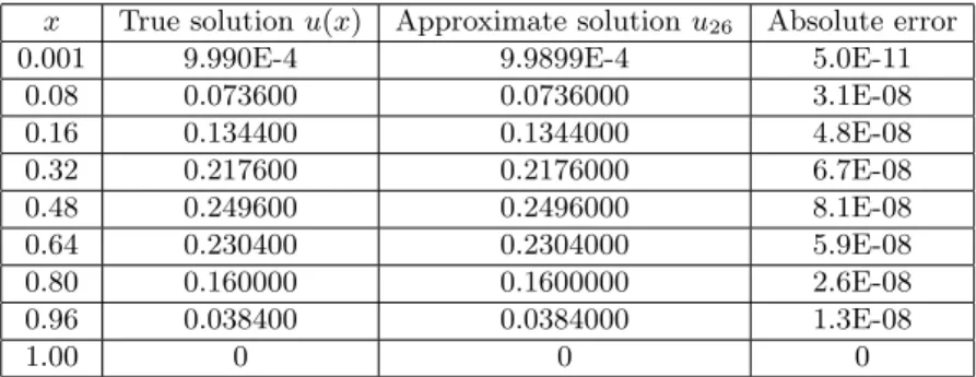
Example 1. Consider the singular equation





u²(x)u⁰⁰(x) + 20u⁰(x)

x³(1 − x)^2.5(x − 0.4)² +sin(u(x)) x√

1 − x = f (x), 0 < x < 1, u(0) = 0, u(1) = 0,

where f (x) = 20−40 x−2 (1−x)^2.5(−1+x)²(−0.4+x)²x⁵+(−1+x)⁴(−0.4+x)²x⁴sin(x−x²) (1−x)⁵²(−0.4+x)²x³ . The true solution is x − x². Using our method, we choose 26 points on [0, 1].

The numerical results are given in the following table 1.

Example 2. Consider the singular equation ( pu(x)u⁰⁰(x) +_sin(x)3(1−x)^30u2.2(x−0.4)^{0(x) 2}(x−0.6)+

√u(x)

1−x = f (x), 0 < x < 1, u(0) = 0, u(1) = 0,

where

f (x) = {csc(x)³ ³

30 π cos(π x) + (1 − x)^1.2 (−0.6 + x) (−0.4 + x)²sin(x)³

× sin(π x) − π²(1 − x)^2.2 (−0.6 + x) (−0.4 + x)²sin(x)³sin(π x)^1.5´ } /{(1 − x)^2.2 (−0.6 + x) (−0.4 + x)²}.

The true solution is sin(πx). Using our method, we choose 26 points on [0, 1].

The numerical results are given in the following table 2.

Example 3. Consider the singular equation





u(x)u⁰⁰(x) + u⁰(x)

x²(1 − x)³ +u²(x)

1 − x = f (x), 0 < x < 1, u(0) = 0, u(1) = 0,

where

f (x) = −1.1752 + cosh(x) + (1 − x)³x²sinh(x) (−1.1752x + sinh(x)) (1 − x)³x²

+(1 − x)²x²(−1.1752 x + sinh(x))³ (1 − x)³x² .

The true solution is sinh(x) − sinh(1)x. Using our method, we choose 26 points on [0, 1]. The numerical results are given in the following table 3.

Table 1. Numerical results for example 1(n = 26).

x True solution u(x) Approximate solution u26 Absolute error

0.001 9.990E-4 9.9899E-4 5.0E-11

0.08 0.073600 0.0736000 3.1E-08

0.16 0.134400 0.1344000 4.8E-08

0.32 0.217600 0.2176000 6.7E-08

0.48 0.249600 0.2496000 8.1E-08

0.64 0.230400 0.2304000 5.9E-08

0.80 0.160000 0.1600000 2.6E-08

0.96 0.038400 0.0384000 1.3E-08

1.00 0 0 0

Table 2. Numerical results for example 2(n = 26).

x True solution u(x) Approximate solution u26 Absolute error

0.001 0.0031415 0.0031414 1.7E-07

0.08 0.2486900 0.2486450 4.4E-05

0.16 0.4817540 0.4817060 4.7E-05

0.32 0.8443280 0.8442490 4.8E-05

0.48 0.9980270 0.9979780 4.8E-05

0.64 0.9048270 0.9047790 4.8E-05

0.80 0.5877850 0.5877370 4.8E-05

0.96 0.1253330 0.1252720 6.0E-05

1.00 0 0 0

Table 3. Numerical results for example 3(n = 26).

x True solution u(x) Approximate solution u26 Absolute error

0.001 -1.7520E-4 -1.7519E-4 1.0E-08

0.08 -0.0139307 -0.0139391 9.4E-06

0.16 -0.0273486 -0.0273614 1.2E-05

0.32 -0.0505750 -0.0505831 8.0E-06

0.48 -0.0654511 -0.0654407 1.0E-05

0.64 -0.0675345 -0.0675128 2.1E-05

0.80 -0.0520550 -0.0520382 1.6E-05

0.96 -0.0137914 -0.0137858 5.5E-06

1.00 0 0 0

5. Appendix

Appendix A. The coefficients of the reproducing kernel Rx(y)

∆₁= 48(−1 + e)e^{3 x}(57121 + 171363e + 287970e²+ 409502e³+ 283644e⁴ +283644e⁵+ 409502e⁶+ 287970e⁷+ 171363e⁸+ 57121e⁹)

∆2= 60 (−1 + e) e^{3 x}(57121 + 114242 e + 173728 e²+ 235774 e³+ 47870 e⁴ +235774 e⁵+ 173728 e⁶+ 114242 e⁷+ 57121 e⁸)

∆3= 5∆1

c1= _∆¹

1(−6318 e⁴− 19548 e⁵− 19548 e⁶− 19548 e⁷− 6318 e⁸− 55926 e^{4 x}

−7648 e^{5 x}+ 6453 e^{6 x}+ 7488 e^3+x+ 30816 e^4+x+ 30816 e^5+x

+57121 e^{2 (5+x)}+ 30816 e^6+x+ 30816 e^7+x+ 7488 e^8+x+ 54756 e^{2+2 x} +108232 e^{3+2 x}+ 165353 e^{4+2 x}+ 222474 e^{5+2 x}+ 39495 e^{6+2 x}

+229764 e^{7+2 x}+ 171363 e^{8+2 x}+ 114242 e^{9+2 x}− 111852 e^{1+4 x}

−167778 e^{2+4 x}− 223704 e^{3+4 x}− 37080 e^{4+4 x}− 223704 e^{5+4 x}

−167778 e^{6+4 x}− 111852 e^{7+4 x}− 55926 e^{8+4 x}− 15296 e^{1+5 x}

−22944 e^{2+5 x}− 46272 e^{3+5 x}− 46272 e^{4+5 x}− 22944 e^{5+5 x}

−15296 e^{6+5 x}− 7648 e^{7+5 x}+ 12906 e^{1+6 x}+ 19359 e^{2+6 x} +32724 e^{3+6 x}+ 19359 e^{4+6 x}+ 12906 e^{5+6 x}+ 6453 e^{6+6 x}) c₂= _∆¹

1(6453 e⁴+ 12906 e⁵+ 19359 e⁶+ 32724 e⁷+ 19359 e⁸+ 12906 e⁹ +6453 e¹⁰+ 57121 e^{4 x}− 7648 e^3+x− 15296 e^4+x− 22944 e^5+x

−55926 e^{2 (5+x)}− 46272 e^6+x− 46272 e^7+x− 22944 e^8+x− 15296 e^9+x

−7648 e^10+x− 55926 e^{2+2 x}− 111852 e^{3+2 x}− 167778 e^{4+2 x}

−223704 e^{5+2 x}− 37080 e^{6+2 x}− 223704 e^{7+2 x}− 167778 e^{8+2 x}

−111852 e^{9+2 x}+ 114242 e^{1+4 x}+ 171363 e^{2+4 x}+ 229764 e^{3+4 x} +39495 e^{4+4 x}+ 222474 e^{5+4 x}+ 165353 e^{6+4 x}+ 108232 e^{7+4 x}

+54756 e^{8+4 x}+ 7488 e^{2+5 x}+30816 e^{3+5 x}+30816 e^{4+5 x}+30816 e^{5+5 x} +30816 e^{6+5 x}+ 7488 e^{7+5 x}− 6318e^{2+6 x}− 19548 e^{3+6 x}

−19548 e^{4+6 x}− 19548 e^{5+6 x}− 6318 e^{6+6 x}) c3= −_∆²

1(1080e⁴− 105840e⁵+ 1080e⁶+ 9560e^4x− 118305e^5x+ 51624e^6x

−1280 e^3+x+ 243745 e^4+x+ 55841 e^5+x+ 60766 e^6+x+ 59486 e^7+x +57121 e^8+x+ 57121 e^9+x− 9360 e^{2+2 x}− 29160 e^{3+2 x}− 9360 e^{4+2 x}

−29160 e^{5+2 x}− 9360 e^{6+2 x}+ 9560 e^{1+4 x}+ 19120e^{2+4 x}+ 38720e^{3+4 x} +19120 e^{4+4 x}+ 9560 e^{5+4 x}+ 9560 e^{6+4 x}− 118305 e^{1+5 x}

−121950 e^{2+5 x}− 121950 e^{3+5 x}− 118305 e^{4+5 x}− 118305 e^{5+5 x} +51624 e^{1+6 x}+ 52704 e^{2+6 x}+ 51624 e^{3+6 x}+ 51624 e^{4+6 x}) c4= −_∆¹

2(51624e⁵+ 51624e⁶+ 52704e⁷+ 51624e⁸+ 51624e⁹+ 57121e^5x

−118305e^4+x−118305e^5+x−121950e^6+x− 121950e^7+x− 118305e^8+x

−118305e^9+x+ 9560e^3+2x+ 9560e^4+2x+ 19120e^5+2x+ 38720e^6+2x +19120e^7+2x+ 9560e^8+2x+ 9560e^9+2x− 9360e^3+4x− 29160e^4+4x

−9360e^5+4x− 29160e^6+4x− 9360e^7+4x+ 57121e^1+5x+ 59486e^2+5x +60766e^3+5x+ 55841e^4+5x+ 243745e^5+5x− 1280e^6+5x+ 1080e^3+6x

−105840e^4+6x+ 1080e^5+6x) c5= _∆¹

3e^−3x(3645e⁴− 179334e⁵− 122213e⁶+ 121532e⁷+ 116607e⁸ +114242e⁹+ 57121e¹⁰+ 32265e^4x− 206496e^5x+ 117110e^6x

−4320e^3+x+ 419040e^5+x− 4320e^6+x− 31590e^2+2x− 97740e^3+2x

−97740e^4+2x− 97740e^5+2x− 31590e^6+2x+ 64530e^1+4x+ 96795e^2+4x +163620e^3+4x+ 96795e^4+4x+ 64530e^5+4x+ 32265e^6+4x

−412992e^1+5x− 417312e^2+5x− 417312e^3+5x− 412992e^4+5x

−206496e^5+5x+ 234220e^1+6x+ 235500e^2+6x+ 234220e^3+6x+ 117110e^4+6x) c₆= _∆¹

3e^−3x(117110e⁶+ 234220e⁷+ 235550e⁸+ 234220e⁹+ 117110e¹⁰ +57121e^6x− 206496e^5+x+ 32265e^10+2x− 412992e^6+x− 417312e^8+x

−412992e^9+x−206496e^10+x+32265e^4+2x+ 64530e^5+2x+ 96795e^6+2x +163620e^7+2x+96795e^8+2x+64530e^9+2x− 31590e^4+4x− 97740e^7+4x

−31590e^8+4x− 4320e^4+5x+ 419040e^5+5x+ 419040e^6+5x− 4320e^7+5x +114242e^1+6x+ 116607e^2+6x+ 121532e^3+6x− 122213e^4+6x

−179334e^5+6x+ 3645e^6+6x) d1= _∆¹

1(−6318e⁴− 19548e⁵− 19548e⁶− 19548e⁷− 6318e⁸+ 57121e^2x

−55926e^4x− 7648e^5x+ 6453e^6x+ 7488e^3+x+ 30816e^4+x

+30816e^5+x+ 30816e^6+x+ 30816e^7+x+ 7488e^8+x+ 114242e^1+2x +171363e^2+2x+ 229764e^3+2x+ 39495e^4+2x+ 222474e^5+2x +165353e^6+2x+ 108232e^7+2x+ 54756e^8+2x− 111852e^1+4x

−167778e^2+4x− 223704e^3+4x− 37080e^4+4x− 223704e^5+4x

−167778e^6+4x− 111852e^7+4x− 55926e^8+4x− 15296e^1+5x

−22944e^2+5x− 46272e^3+5x− 46272e^4+5x− 22944e^5+5x

−15296e^6+5x− 7648e^7+5x+ 12906e^1+6x+ 19359e^2+6x +32724e^3+6x+ 19359e^4+6x+ 12906e^5+6x+ 6453e^6+6x) d2= _∆¹

1e^{2−3 x}(6453 e²+ 12906 e³+ 19359 e⁴+ 32724 e⁵+ 19359 e⁶ +12906 e⁷+ 6453 e⁸− 55926 e^{2 x}+ 54756 e^{4 x}+ 7488 e^{5 x}− 6318 e^{6 x}

−7648 e^1+x− 15296 e^2+x− 22944 e^3+x− 46272 e^4+x− 46272e^5+x

−22944e^6+x− 15296e^7+x− 7648e^8+x− 111852e^{1+2 x}− 167778e^{2+2 x}

−223704e^{3+2 x}− 37080e^{4+2 x}− 223704 e^{5+2 x}− 167778 e^{6+2 x}

−111852 e^{7+2 x}− 55926 e^{8+2 x}+ 108232 e^{1+4 x}+ 165353 e^{2+4 x} +222474 e^{3+4 x}+ 39495 e^{4+4 x}+ 229764 e^{5+4 x}+ 171363 e^{6+4 x} +114242 e^{7+4 x}+ 57121 e^{8+4 x}+ 30816 e^{1+5 x}+ 30816 e^{2+5 x} +30816 e^{3+5 x}+ 30816 e^{4+5 x}+ 7488 e^{5+5 x}− 19548e^{1+6 x}

−19548 e^{2+6 x}− 19548 e^{3+6 x}− 6318 e^{4+6 x}) d3= −_∆¹

2(1080e⁴− 105840e⁵+ 1080e⁶+ 57121e^x+ 9560e^4x− 118305e^{5 x} +51624e^6x+ 57121 e^1+x+ 59486 e^2+x+ 60766 e^3+x+ 55841 e^4+x +243745 e^5+x− 1280 e^6+x− 9360 e^{2+2 x}− 29160 e^{3+2 x}− 9360 e^{4+2 x}

−29160 e^{5+2 x}− 9360 e^{6+2 x}+ 9560 e^{1+4 x}+ 19120 e^{2+4 x} +38720 e^{3+4 x}+ 19120 e^{4+4 x}+ 9560 e^{5+4 x}+ 9560 e^{6+4 x}

−118305 e^{1+5 x}− 121950 e^2+5x− 121950 e^{3+5 x}− 118305 e^{4+5 x}

−118305 e^{5+5 x}+ 51624 e^{1+6 x}+ 52704 e^{2+6 x}+ 51624 e^{3+6 x} +51624 e^{4+6 x})

d₄= −_∆¹

2e^{3−3 x}(51624 e²+ 51624 e³+ 52704 e⁴+ 51624 e⁵+ 51624 e⁶ +9560 e^{2 x}− 9360 e^{4 x}− 1280 e^{5 x}+ 1080 e^{6 x}− 118305 e^1+x

−118305 e^2+x− 121950 e^3+x− 121950 e^4+x− 118305 e^5+x

−118305 e^6+x+ 9560 e^{1+2 x}+ 19120 e^{2+2 x}+ 38720 e^{3+2 x} +19120 e^{4+2 x}+ 9560 e^{5+2 x}+ 9560 e^{6+2 x}− 29160 e^{1+4 x}

−9360 e^{2+4 x}− 29160 e^{3+4 x}− 9360 e^{4+4 x}+ 243745 e^{1+5 x} +55841 e^{2+5 x}+ 60766 e^{3+5 x}+ 59486 e^{4+5 x}+ 57121 e^{5+5 x}

+57121 e^{6+5 x}− 105840 e^{1+6 x}+ 1080 e^{2+6 x}) d₅= _∆¹

3e^−3x(57121 + 114242e + 116607e²+ 121532e³− 122213e⁴

−179334e⁵+ 3645e⁶+ 32265e^4x− 206496e^5x+ 117110e^6x

−4320e^3+x+ 419040e^4+x+ 419040e^5+x− 4320e^6+x− 31590e^2+2x

−97740e^3+2x− 97740e^4+2x− 97740e^5+4x− 31590e^6+2x +64530e^1+4x+ 96795e^2+4x+ 163620e^3+4x+ 96795e^4+4x +64530e^5+4x+ 32265e^6+4x− 412992e^1+5x− 417312e^2+5x

−417312e^3+5x− 412992e^4+5x− 206496e^5+5x+ 234220e^1+6x +235550e^2+6x+ 234220e^3+6x+ 117110e^4+6x)

d6= _∆¹

3e^4−3x(117110e²+ 234220e³+ 235500e⁴+ 234220e⁵+ 117110e⁶ +32265e^2x− 31590e^4x− 4320e^5x+ 3645e^6x− 206496e^1+x

−412992e^2+x− 417312e^3+x− 417312e^4+x− 412992e^5+x

−206496e^6+x+ 64530e^1+2x+ 96795e^2+2x+ 163620e^3+2x +96795e^4+2x+ 64530e^5+2x+ 32265e^6+2x− 97740e^1+4x

−97740e^2+4x− 97740e^3+4x− 31590e^4+4x+ 419040e^1+5x +419040e^2+5x− 4320e^3+5x− 179334e^1+6x− 122213e^2+6x +121532e^3+6x+ 116607e^4+6x+ 114242e^5+6x+ 57121e^6+6x)

Appendix B. The proof of Theorem 2.1 Through several integrations by parts for (2.1), then (B.1)

(u(y), R_x(y))_W3 2

= R₁

0 u(y)(36Rx(y) − 49R⁽²⁾x (y) + 14R⁽⁴⁾x (y) − R⁽⁶⁾x (y))dy + u(y)(49R⁰_x(y)

−14R⁽³⁾x (y) + R⁽⁵⁾x (y))|¹₀+ u⁰(y)(14R⁽²⁾x (y) − R⁽⁴⁾x (y))|¹₀+ u⁰⁰(y)R⁽³⁾x (y)|¹₀. Since Rx(y) ∈ W₂³[0, 1], it follows that

Rx(0) = 0, Rx(1) = 0.

(B.2)

Since u ∈ W₂³[0, 1], u(0) = u(1) = 0. If (B.3)

14R⁽²⁾_x (0) − R⁽⁴⁾_x (0) = 0, 14R_x⁽²⁾(1) − R⁽⁴⁾_x (1) = 0, R⁽³⁾_x (0) = 0, R⁽³⁾_x (1) = 0, then (B.1) implies that

(u(y), Rx(y))_W³

2 =

Z ₁

0

u(y)(36Rx(y) − 49R⁽²⁾_x (y) + 14R⁽⁴⁾_x (y) − R⁽⁶⁾_x (y))dy.

For ∀x ∈ [0, 1], if Rx(y) also satisfies

(B.4) 36Rx(y) − 49R⁽²⁾_x (y) + 14R⁽⁴⁾_x (y) − R⁽⁶⁾_x (y) = δ(y − x), then

(u(y), Rx(y))_W³

2 = u(x).

Characteristic equation of (B.4) is given by

λ⁶− 14λ⁴+ 49λ²− 36 = 0,

then we can obtain characteristic values λ1= 1, λ2= −1, λ3= 2, λ4= −2, λ5= 3, and λ6= −3. So, let

Rx(y) =

½ c1e^y+ c2e^−y+ c3e^2y+ c4e^−2y+ c5e^3y+ c6e^−3y, y ≤ x, d1e^y+ d2e^−y+ d3e^2y+ d4e^−2y+ d5e^3y+ d6e^−3y, y > x.

On the other hand, for (B.4), let Rx(y) satisfy

(B.5) R^(k)_x (x + 0) = R^(k)_x (x − 0), k = 0, 1, 2, 3, 4.

Integrating (B.4) from x − ε to x + ε with respect to y and let ε → 0, we have the jump degree of R⁽⁵⁾x (y) at y = x

(B.6) R⁽⁵⁾_x (x − 0) − R⁽⁵⁾_x (x + 0) = 1.

From (B.2), (B.3), (B.5), (B.6), the unknown coefficients of (2.2) can be ob- tained.

References

[1] R. P. Agarwal and D. O’Regan, Second-order boundary value problems of singular type, J. Math. Anal. Appl. 226 (1998), no. 2, 414–430.

[2] M. K. Kadalbajoo and V. K. Aggarwal, Numerical solution of singular boundary value problems via Chebyshev polynomial and B-spline, Appl. Math. Comput. 160 (2005), no. 3, 851–863.

[3] P. Kelevedjiev, Existence of positive solutions to a singular second order boundary value problem, Nonlinear Anal. 50 (2002), no. 8, Ser. A: Theory Methods, 1107–1118.

[4] C. Li and M. Cui, The exact solution for solving a class nonlinear operator equations in the reproducing kernel space, Appl. Math. Comput. 143 (2003), no. 2-3, 393–399.

[5] Y. Liu and A. Qi, Positive solutions of nonlinear singular boundary value problem in abstract space, Comput. Math. Appl. 47 (2004), no. 4-5, 683–688.

[6] Y. Liu and H. Yu, Existence and uniqueness of positive solution for singular boundary value problem, Comput. Math. Appl. 50 (2005), no. 1-2, 133–143.

[7] R. K. Mohanty, P. L. Sachdev, and N. Jha, An O(h⁴) accurate cubic spline TAGE method for nonlinear singular two point boundary value problems, Appl. Math. Com- put. 158 (2004), no. 3, 853–868.

[8] A. S. V. Ravi Kanth and Y. N. Reddy, Higher order finite difference method for a class of singular boundary value problems, Appl. Math. Comput. 155 (2004), no. 1, 249–258.

[9] , Cubic spline for a class of singular two-point boundary value problems, Appl.

Math. Comput. 170 (2005), no. 2, 733–740.

[10] J. Wang, W. Gao, Z. Zhang, Singular nonlinear boundary value problems arising in boundary layer theory, J. Math. Anal. Appl. 233 (1999), no. 1, 246–256.

[11] X. Xu and J. Ma, A note on singular nonlinear boundary value problems, J. Math.

Anal. Appl. 293 (2004), no. 1, 108–124.

[12] X. Zhang and L. Liu, Positive solutions of superlinear semipositone singular Dirichlet boundary value problems, J. Math. Anal. Appl. 316 (2006), no. 2, 525–537.

Fazhan Geng

Department of Mathematics Harbin Institute of Technology Weihai, Shandong, P. R. China Minggen Cui

Department of Mathematics Harbin Institute of Technology Weihai, Shandong, P. R. China E-mail address: [email protected]