Vol. 66, No. 5, May 2016, pp. 545∼550 http://dx.doi.org/10.3938/NPSM.66.545
Water NMR for Polarized
129Xe Signal Calibration with a 283 G Magnetic Field
Vladimir Vladimirovich Kavtanyuk · Joshua Artem Tan · Wooyoung Kim
∗· Yonggeun Seon · Seongwoo Park · Jieun So · Yu Ando
Department of Physics, Kyungpook National University, Daegu 41566, Korea (Received 14 December 2015 : revised 11 January 2016 : accepted 11 January 2016)
We present measurements of water nuclear magnetic resonance (NMR) for polarized129Xe signal calibration. We used a permanent magnet having an average homogeneous space in the center and a field of 283±2 G. A Pick-up coil was orthogonally inserted inside the RF coil. Oscillating RF and pick-up signals were managed by using Tecmag Apollo LF-1. Two LC circuits (the RF and the pick-up) were set to a resonance frequency of 1.205 MHz by manipulating a capacitance system.
The nuclear spins of the protons in water are flipped and precess with the Larmor frequency around the direction of the static field. Tha application of an oscillating magnetic field with the Larmor frequency perpendicular to the static magnetic field leads to resonance absorption and emission of the electromagnetic energy. The emitted resonance signals are acquired by the pick-up coil and sent to the Apollo for analysis. In the future, the water NMR signal will be used for determining the polarization of129Xe.
PACS numbers: 21.10.Hw
Keywords: Water NMR, Polarized129Xe
I. INTRODUCTION
The necessity for polarized gases in medicine comes from the absence of a convenient medium in lung spaces with which to perform magnetic resonance imaging (MRI). The low density of protons in the lungs gives very small signal when performing MRI. Motion cor- rection is also not suitable using proton MRI to study the lungs. Administering a polarized gas to a patient, provides a high signal NMR medium with which to im- age their lungs and air spaces and make quantitative measurements of these spaces. Moreover, polarized gases have also found uses in material and particle physics in- cluding the determination of the neutron spin structure function measured by scattering polarized high energy electrons from highly polarized targets of3He [1], stud- ies of surface interactions [2,3], studies of fundamental
∗E-mail: [email protected]
symmetries [4,5], and neutron polarizers and polarime- ters [6]. For lung studies and neutron filters, polarized
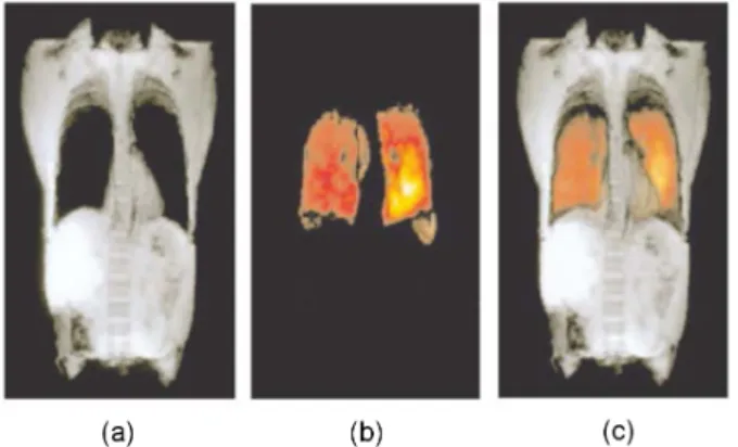
3He has been used widely. However the limited global supply of3He (a by-product of tritium decay) will pre- clude the large scale introduction of polarized 3He as a medical diagnostic medium in MRI. 129Xe has many advantages over3He including an almost unlimited sup- ply (it is naturally abundant), its solubility in a large range of solutions, and high absorption rates onto ma- terial surfaces. This makes 129Xe ideal as a functional MRI medium for lung spaces and for the characteriza- tion of porous media using MRI. Fig. 1 shows the first spin-density human lung image, obtained at University of Virginia after collaboration with the Princeton group, responsible with the production of polarized xenon. The image was acquired in a healthy volunteer using 71%
enriched xenon [7].
The nuclear spin of the protons in a static magnetic field, gets flipped and precesses around the direction of
This is an Open Access article distributed under the terms of the Creative Commons Attribution Non-Commercial License (http://creativecommons.org/licenses/by-nc/3.0) which permits unrestricted non-commercial use, distribution, and reproduction in any medium, provided the original work is properly cited.
Fig. 1. (Color online) First human lung image ac- quired with hyperpolarized xenon: (a) Proton MRI im- ages showing no signal over the lung space, (b) Polarized
129Xe MRI image showing excellent resolution over the lung space filled with gas, and (c) The first two images superposed. Adapted from [8].
the field ⃗B0 with the Larmor frequency:
f = γB0, (1)
where γ is the gyromagnetic ratio (γwater = 4.257 kHz/G, γ129Xe = 1.18 kHz/G) and B0 is the magni- tude of the static magnetic field. An oscillating magnetic field, which is perpendicularly applied to the direction of the static field with the same resonance frequency as the Larmor frequency, provides a flip of the spins around the static field inducing electric signal to the surround- ing coils. Water is used, for calibration, as the unit of the polarization, because its polarization can be easily calculated as [9]:
P = tan hB0µ
kBT, (2)
where P is the polarization, kB is the Boltzmann con- stant, T is the temperature, and µ is the magnitude of the magnetic moment of the spin [7]. It comes from the relationship between the number of spins in the lower energy level N− and number of spins in the high energy level N+ described by Boltzmann statistics as:
N+= N−ekBT∆E , (3) where ∆E is the energy difference [10] which is equivalent to 2µB0for S=1/2 spins immersed in the static magnetic field of magnitude B0, and the definition of polarization:
P = N+− N−
N++ N−. (4)
where P is the polarization, S is the signal strength equal to the peak of the Fourier transform (FT), and N is the number of nuclei. The number of xenon atoms is calculated based on the ideal gas law:
NXe= PXeV
kBTXeβ129, (6) where PXe is the xenon partial pressure in the gas mix- ture, V is the sensitive volume of the Pick-up coil, and TXeis the gas mixture temperature considered to be the room temperature. The isotopic abundance β129is 26.4%
for the natural xenon. The number of protons in a water sample is calculated as:
NH= 2V NAρwater
18 , (7)
where V is the same active volume of the Pick-up coil, NA is Avogadro’s number, 18 is the molecular mass of water (in AMU), ρwater is the density of water, and 2 is the number of protons per water molecule [7].
The measurements of water NMR were performed in time domain first, where we could see a free education decay (FID) signal of water, then the time domain was switched to frequency domain by using the Fourier trans- form. FID is the observable NMR signal generated by non-equilibrium nuclear spin magnetization precessing about the magnetic field.
II. EXPERIMENT
1. Permanent Magnet
The permanent magnet consists of two parallel mag- netic plates, which are fixed to each other at the bottom by a metallic holder as shown on the Fig. 2. There is a homogeneous space, 3 cm× 3 cm × 3 cm, in the center of the permanent magnet, which provides the magnetic field 283± 2 G.
Fig. 2. A schematic view of the permanent magnet with 20.2 cm high, 15 cm wide, and 15 cm thick.
Fig. 3. (Color online) The RF and the Pick-up coils.
2. NMR Coils
Two solenoids, which were made by hands, were used as NMR coils (Fig. 3). One was made for the RF circuit, and another for the Pick-up circuit.The specification of the RF coil is the following: 1 winding layer, 35 mm length, 33 windings, 1 mm wire diameter, and 48 mm diameter. The Pick-up coil has 2 layers, 0.8 mm length, 20 windings, 0.32 mm wire diameter, and 32 mm diam- eter.
3. LC Circuits and Capacitance System
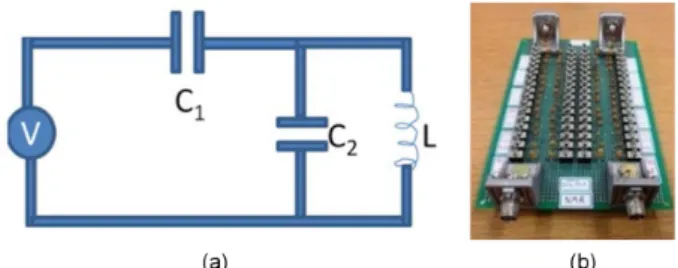
LC circuit, also called the resonant circuit, is an elec- tric circuit consisting of an inductor and capacitors. By manipulating the C1 and the C2 capacitance decade boxes, we can set the resonance frequency. A capacitance decade box is basically just parallel connected capacitors with switches. Fig. 4.a shows the LC circuit which was
Fig. 4. (Color online) (a) LC circuit diagram, where V is a voltage source (Tecmag Apollo LF-1), L is a NMR coil, and C1 and C2 are capacitance decade boxes, (b) the capacitance system.
used in the experiment, one for the RF coil, and another, which is exactly same, was used for the Pick-up coil.
The capacitance system includes 4 capacitance decade boxes, which were made on one plate for convenience (Fig. 4(b)). Each of the capacitance decade boxes has a capacitance range 0.5 pF to 3500 pF. The relationship between resonance frequency, capacitance, and induc- tance is expressed by the following formula:
f =
√
1
4π2L(C1 + C2). (8)
4. Tecmag Apollo LF-1, HP Network analyzer 4195 A, Amplifier LZY-22+, and Pre-amplifier AU- 1147.
Tecmag Apollo LF-1 is a compact, modular, Windows based console which is configurable from 2 kHz to 100 MHz. The Apollo plays an important role in our ex- periment; it can produce specific RF signals and observe NMR signals using NTNMR software, which is powerful instrument control software. NTNMR is preconfigured for applications and includes an application specific pulse sequence for water and others [11].
A network analyzer is an instrument that measures the network parameters of electrical networks. In the exper- iment, HP Network analyzer 4195 A has been used for monitoring adjustments of the resonance frequency, and determining the Q-factor. 4195 A is a high-performance, and cost-effective analyzer with combined vector network and spectrum analysis capabilities. The frequency is cov- ered from 10 Hz to 500 MHz with an excellent 0.001 Hz resolution [12].
Fig. 5. (Color online) Schematic of the procedure for adjusting resonance frequency.
Amplifier LZY-22+ has been used for increasing the RF signals. This High Power Amplifier has a 24 V / 5.5 A DC power supply and is capable of delivering 30 W output signal across its entire operating bandwidth, 0.1 - 200 MHz. Extensive safety features to prevent ampli- fier damage include over-temperature protection and the ability to handle short and open loads. The LZY-22+
includes heat-sink and cooling fan [13].
The Miteq AU-1447 is a Pre-amplifier with operating frequency range 0.001 to 400 MHz, with gain of 60 dB.
This pre-amplifier has been used for increasing signals from the Pick-up coil [14].
5. Setting the Resonance and Q-factors of the RF and the Pick-up Circuits
Before starting actual water NMR measurements, we had to adjust the RF and the Pick-up circuits to the res- onance frequency of 1.205 MHz. The resonance and Q- factors were set separately for the RF circuit, and for the Pick-up circuit. Fig. 5 shows the procedure for adjusting resonance frequency. By manipulating the capacitance decade boxes, we can set to the resonance frequency and see it directly on the Network analyzer’ s screen. The BNC cables, which were used in the procedure, have 50 Ohm impedance.
Q-factor or the quality factor is a dimensionless param- eter that characterizes a resonator’ s bandwidth relative to its center frequency. Q-factor can be changed by ma- nipulating the C1 and the C2 capacitance decade boxes.
The calculation of the Q-factor is based this simple for- mula:
Q = f
|f1 − f2|, (9)
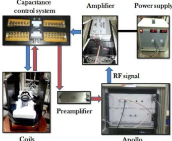
Fig. 6. (Color online) The schematic of the experimental procedure. The blue arrows represent the flow of the output signal, and the red arrows represent the flow of the input signal.
where f is the resonance frequency, f 1 and f 2 are fre- quencies corresponding to a half of the electrical power on the left and the right side of a signal’ s peak. Q-factor for the RF coil was 38 and for the Pick-up coil was 46.
The information on frequencies, which represent half of the electrical power, can be easily seen on the Network analyzer’ s screen.
6. Experimental Method
Before setting the resonance frequency and the Q- factors of the RF and the Pick-up circuits, the RF coil was placed in the center of the permanent magnet so that their magnetic fields would be perpendicular. The Pick-up coil was positioned perpendicular inside the RF coil. A small paper cup was placed in the middle of the Pick-up coil to hold water. Fig. 6 shows the schematic of the experimental procedure. The Apollo sends the RF signal with 1.205 MHz to the amplifier, and then the amplified signal goes through the capacitance system to the RF coil. The Pick-up coil captures the resonance signal from water, and it goes through the preamplifier to the Apollo for observation. The experiment was per- formed with 20 scans with water, and without water, so it would be possible to distinguish water NMR signal from the ringdown signal: the decaying electrical oscillation
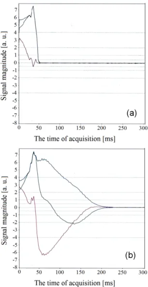
Fig. 7. (Color online) Comparison between background and water NMR signal in the time domain: a) the back- ground, b) the background plus FID signal of water. The y-axis scales the magnitude of the signal in arbitrary units and the x-axis corresponds to the time of acquisi- tion in milliseconds.The red line represents real part, the green is imaginary, and the blue is magnitude.
of the RF circuit. The adjustments of the resonance fre- quency had to be performed every time water was filled or taken out from the paper cup using the network an- alyzer, since the presence or the absence of water gave a resonance shift due to impedance’ s changes in the RF and the Pick-up circuits.
The NTNMR software, which we used, added scan re- sults to each other, so it means that the result was a sum of the 20 scans (not average). The experiment was per- formed several times to confirm the stability of the water signal, since it plays an important role in the calculation
Fig. 8. (Color online) Comparison between background and water NMR signal in the frequency domain: a) the background, b) the background plus water NMR signal.
The y-axis corresponds to the signal magnitude in ar- bitrary units and x-axis has the dimension of frequency, kHz. The red line represents real part, the green is imag- inary, and the blue is magnitude.
of the129Xe polarization. The water signal was observed at 45,000± 1,000 a.u., every time we measured it, which shows the good stability.
III. RESULTS AND DISCUSSION
NMR signals were obtained with the empty cup and with the cup filled with water. These signals correspond to the background signal and the water NMR signal, re- spectively. The free education decay (FID) signal was clearly distinguished from the noise and the ring-down signal (Fig. 7). The comparison of the background and water NMR signal showed significant difference. After the Fourier transform of these signals, the ringdown sig- nal showed a peak at about 6,000 a.u., and the ringdown + water is about 45,000 a.u. (Fig. 8). This difference in the peaks was associated with a pure water signal which is about 39,000 a.u. for the 20 scans.
between the background and the water signal is about 39,000 a.u., which represents a pure water NMR signal, obtained with the 20 scans. The experimental method of detecting water NMR signal was well established, and this technique will be very useful, in the future, for mea- suring129Xe polarization.
ACKNOWLEDGEMENTS
This work was supported by the National Re- search Foundation of Korea under Grant No. NRF- 2013R1A2A2A01016502. This work was also supported by Kyungpook National University Research Fund, 2012.
REFERENCES
[1] P. L. Anthony, R. G. Arnold, H. R. Band, H. Borel and P. E. Bosted et al., Phys. Rev. Lett., 71, 959 (1993).
[2] Z. Wu, W. Happer, M. Kitano and J. Daniels, Phys.
Rev. A 42, 2774 (1990).
[3] D. Raftery, H. Long, T. Meersmann, P. J.
Grandinetti and L. Reven et al., Phys. Rev. Lett.
66, 584 (1991).
J. DeAngelis and G. E. Dodge et al., Phys. Rev.
Lett. 68, 2901 (1992).
[7] I. C. Ruset, Ph. D. thesis, University of New Hamp- shire, 2005.
[8] J. P. Mugler III, B. Driehuys, J. R. Brookeman, G.
D. Cates and S. S. Berr et al., Magn. Res. Med. 37, 809 (1997).
[9] J. A. Tan, V. Kavtanyuk, Y. Seon and W. Kim, New Phys.: Sae Mulli 64, 131 (2014).
[10] J. P. Hornak, The Basics of NMR (www.cis.rit.edu/
htbooks/nmr, 1997-99), Chap. 3, 6.
[11] Model LF-1, Tecmag Inc., Houston, TX, http:// tec- mag.com/apollo.html (accessed on Nov. 30, 2015).
[12] Model 4195 A, Hewlett-Packard Inc., Miami, FL, http://wiki.epfl.ch/carplat/documents/PDF/
HP4195A.pdf (accessed on Nov. 30, 2015).
[13] Model LZY-22+, Mini-Circuits Inc., Brooklyn, NY, http://www.minicircuits.com/pdfs/LZY-22+.pdf (accessed on Nov. 30, 2015).
[14] Model AU-1447, Miteq inc., Hauppauge, NY, https://www.miteq.com/viewmodel.php?model=AU- 1447 (accessed on Nov. 30, 2015).