Audio Signal Processing using Parametric Array with KZK Model

(1)

*정회원, 제주대학교 해양시스템공학과

**정회원, (주) 알고코리아

***정회원, 국방과학연구소

접수일자 2009.9.１, 수정일자 2009.10.２

논문 2009-5-20

KZK 모델을 이용한 파라메트릭 어레이 음향 신호 처리

Audio Signal Processing using Parametric Array with KZK Model

이종현^*, Mano Samuel^**, 이재일^*, 김원호^***, 배진호^*

Chong-Hyun Lee, Mano Samuel, Jea-Il Lee, Won-Ho Kim, Jin-Ho Bae

요 약 본 논문에서는 파라메트릭 어레이를 이용한 음향신호에 대한 수치 모델링 기법 및 분석 결과를 제시한다. 사용된 음성 파라메트릭 배열의 분석 수치모델은 KZK(Khokhlov-Zabolotskaya-Kuznetsov)로서 KZK수치모델은 시간 영역의 차분방정식 알고리즘을 사용하며 파라메트릭배열의 정확한 응답특성이 분석이 가능하다. 시간영역기반의 KZK 모델은 음원의 크기와 전송주파수의 영향을 받으며, 가청신호응답은 출력레벨과 빔폭의 크기를 포함한다. 음성신호에 대하여 파라메트릭 배열을 효율적으로 적용시키기 위해서는 고려해야할 요소는 표본화 주파수, 트랜스듀서의 반경 및 변조방식 파라미터 등이 있다. 본 논문에서는 다양한 요소 중 표본화 주파수에 따른 응답신호의 왜곡 분석 및 실험 결과를 시뮬레이션을 통해 제시하였다.

Abstract Parametric array for audio applications is analyzed by numerical modeling and analytical approximation. The nonlinear wave equations are used to provide design guidelines for the audio parametric array. A time domain finite difference code that accurately solves the KZK (Khokhlov-Zabolotskaya-Kuznetsov) nonlinear parabolic wave equation is used to predict the response of the parametric array. The time domain code relates the source size and the carrier frequency to the audible signal response including the output level and beamwidth to considering the implementation issues for audio applications of the parametric array, the emphasis is given to the frequency response and distortion. We use the time domain code to find out the optimal parameters that will help produce the parametric array with highest achievable output in terms of the average power within the demodulated signal. Parameters such as primary input frequency, audio source radius and the modulation method are given utmost importance. The output effect of those parameters are demonstrated through the numerical simulation.

Key Ｗords : Parametric array, KZK model, Numerical modeling, Analytical approximation

Ⅰ. Introduction

The parametric array is a nonlinear transduction mechanism that generates narrow, nearly sidelobe free beams of low frequency sound, through the mixing and

interaction of high frequency sound waves, effectively overcoming the diffraction limit(a kind of spatial 'uncertainty principle') associated whit linear acoustics.

Westervelt presented a theoretical model of the parametric array[1]. The parametric array produces high amplitude ultrasonic waves which demodulate into directional audible sound duehichthe nonlinear characteristics of the medium through which they travel. As a result, a highly directional beam is

(2)

produced. One of the m wavreasons why parametric array is desired is becaituda parametric array produces a secondasonsound beam with similar directivityhichtha directewavreasoncarria hbeam. This is the factor that results in the parametric array producing a low frequency, low beamwidth output.

An input audio signal of frequency _ _when amplitude modulated with a frequency _ _{and passed} through a medium, the modulated output gets demodulated to produce the difference fequency

_ _, the audio signal, due to the self-demodulation characteristics of the medium through which it is traveling. The self- demodulation of the signal occurs due to the nonlinear characteristis of air [1] There have been various studies conducted on this self-demodulation process.

Although there is no closed form solution to the Khokhlov-Zabolotskaya-Kuznetsov (KZK) equation, to emphasize on the mathematical representation of this parametric array, various mathematical models have been proposed to design the nonlinear characteristics.

But one of the most accurate models is th KZK nonlinear wave equation model. The KZK model is known to describe, to the highest degree of accuracy possible, the combined effects of absorption, diffraction and nonlinearity. Here we use the following model to study the characteristics of the parametric audio array.

Ⅱ. The KZK Model

The KZK nonlinear parabolic wave equation is known to very accurately describe the propagation of a finite amplitude sound beam by combining the effects of absorption, diffraction and nonlinearity. In the derivation of the KZK equation, the sound waves are assumed to form a highly directive beam. Although there are no explicit analytical solutions for the KZK equation, many research groups in pursuit of designing a nonlinear wave propagation model have developed a spectral method, a frequency domain approach or an

incomplete time domain model. But Lee[2] developed a time domain algorithm that solves the KZK nonlinear parabolic wave equation for axisymmetric finite amplitude sound beams. We use this time domain algorithm to model a parametric communication system by transmitting an amplitude modulated signal into the time domain code and receiving the demodulated output at a distance x, in the farfield

The KZK equation is an extension of the Burgers equation. This accounts for the combined effects of nonlinearity, absorption and diffraction.

Directive radiation

z y

Axisymmetric source x

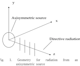
Fig. 1. Geometry for radiation from an axisymmetric source

Let z be the axis along which the beam propagates and let(x,y) be the coordinates perpendicular to the axis. It is known that there is no definite analytical solution to the KZK equation. There with certain assumptions, we use the time domain algorithm here to study and analyze the wave propagation in a nonlinear medium. In regard to the source, certain assumptions that are made are follows: (1) it is defined in the plane z = 0, (2) it has characteristic radius a, (3)it radiates frequencies that satisfy the relation,ka >> 1, (4) the beam emitted by the source is highly directional

Linear theory for directional beams, reveal the existence of near-field and far-field regions. Far-field does not start at a fixed point. The far-field is roughly based on the Rayleigh distance, which is dependent on the carrier frequency involved. The nearfield is characterized by wavefronts that are mostly planar and

(3)

the far field wavefronts, spherical. This is due to the fact that the waves tend to spread out in the far field as the power of the highly directional beam starts to reduce as it propagates along the z axis.

The KZK equation is given by,

^

  _

 ∇^_⊥  

^_

^

^  

_^_

^^

^ (1) Where, ∇_⊥^  ^^ ^^ is a laplacian that operates in the plane perpendicular to the axis of the beam. In order to improve the computational efficiency in the farfield, a co-ordinate transformation is applied to the KZK equation. This transformation provides the geom pry that follows the spherical spreading of the beam in the farfield. The time domain algorithm that we use here solves the KZK equation in a sequence at each range step. First the diffraction term is integrated, then the absorption term and eventually the nonlinear term.

The variable transformations are as follows,

  __

  

  

  _^  ^

   ⁽²⁾

    

where,  radius of the source,    is a dimensionless range co-ordinate in terms of Rayleigh distance, _ _^_ at the characteristic angular frequency, _,  is dimensionless transverse co-ordinate,  is dimensionless retarded time,  is characteristic source pressure amplitude and  _is acoustic pressure.

Thus using the time domain algorithm of the KZK equation, we observe the parametric array’s path along the axis of the beam. Now from the KZK equation, Berktay’s result, the demodulated secondary frequency

pressure, has already been derived as shown in Lee’s dissertation. This Berktay’s result is given as,

_^  ^_^

__^_

^^

^ ⁽³⁾

where  is co-efficient of nonlinearity,  is attenuation co-efficient_ is density of the propagation medium,   is axial distance from the source, _ _is speed of sound in air  is envelope function.

In order to get the demodulated output, we input the preprocessed modulated data into the KZK equation.

The input parameters for the KZK model are given in Table.1.

Table.1 Ideal input parameters

Parameter Value

Sample Frequency > 105 kHz Input source radius 30 cm

Carrier Frequency > 45 kHz

Now we have a continuous source waveform as the input, the amplitude modulated signal, to the KZK model. For example, let us assume a single tone frequency of 4000 Hz is amplitude modulated with a 20 kHz carrier tone. This amplitude modulated signal will serve as the input to the KZK model. △ _{is the} transverse step size. The△ value is normally taken to be 0.03. _ should be in the range of 12>_

> 8 as stated by Lee based on experimental results.

Here for the KZK model, a value of 10 for _ _was chosen. The value of△ _and_ remains the same throughout all simulations.

The ‘△’ value is based on the formula,

△    

  ≤  ≤ 

  ≤  ≤ 

(4)

In our simulations, we settled for a△ value based

(4)

on the Goldberg number obtained. Since the Goldberg number is dependent on the absorption co-efficient which in turn is dependent on the carrier frequency, the

△ value keeps changing based on the input signal considered.

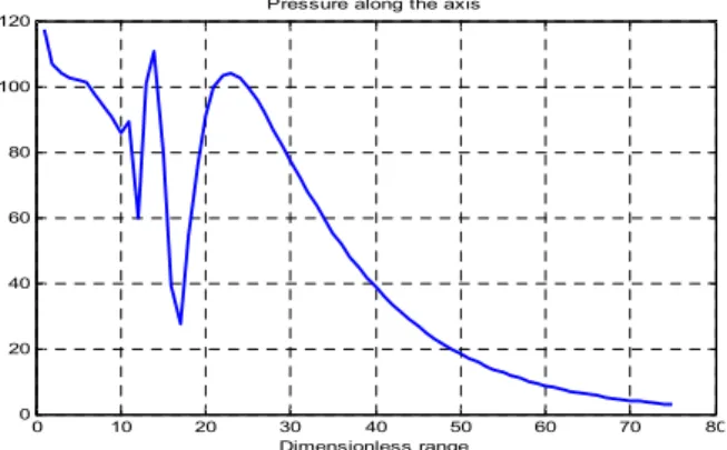
In order to observe the propagation of a wave along the axis of the beam, we need to specify ‘Sigma ‘points or ‘ watch points’. The distance between each point is determined by the step size. There are two methods based on which the step size is designed. The discontinuity in the source’ step function results in numerical oscillations in the nearfield as can be seen in Fig.2.

0 10 20 30 40 50 60 70 80

0 20 40 60 80 100 120

Dimensionless range

Dimensionless pressure

Pressure along the axis

Fig. 2 Propagation of a beam along the axis

In order to overcome these oscillations, we opt for an Implicit Backward Finite Difference (IBFD) method which is effective in damping the oscillations. The downside to this is the fact that the IBFD method requires small step sizes for accurate results. The step size (△) used here is .001. As mentioned before, smaller step sizes translate into higher computation time. The self-demodulation of the signal is quite an interesting study that has its applications in various fields. Companies such as Holosonics and ATC have been able to exploit this feature to commercialize products that produce high directivity output. Now how does a modulated signal automatically get demodulated? Consider this. The source condition for a piston is given by,

         

          ⁽⁵⁾

where, amplitude modulation   _{and phase} modulation   are slowly varying functions of time.

As already mentioned earlier, we consider the attenuation co-efficient to be large enough (_≥ ) to contain the non-linear interaction in the nearfield based on the Rayleigh Distance. The instantaneous angular frequency of the carrier wave is

     . Based on the parametric array model, the primary beam is considered to be a collimated plane wave, and further assume that the exponential attenuation acts locally based on the instantaneous angular frequency :

_  ≃ _^{  } _       (6)

The frequency content of the secondary pressure,

_, based on the difference frequency, is determined by,

^_. The high frequency spectrum is absorbed more rapidly than the low frequency spectrum. Therefore most, or all of the output is based on the low frequency spectrum contribution which is given by,

^_  ≃ 

^_^{   }^     (7)

The length of the non-linear interaction region itself is given by,

_ _^{ } (8)

A further assumption is made that the absorption of the nonlinearly generated low-frequency components is a relatively weak effect, which is justified if  _and

   are slow varying functions of time, corresponding to the very low frequencies. The wave

(5)

equation for _ _becomes,

_

  _

 

 ∞



∇^_⊥_  

_^_

^_

  (9)

Using Fourier transforms and the definition of Green’s function, one finds that the solution for the demodulated output along the axis of the beam for arbitrary _  _is,

   

^

^

^







∞

^^^  ^

  ^{ }^^^

  ^ (10)

Substituting Eq.7 into Eq.10 yields,

_   ^_^

_^_

^

^

^ 

    (11)

For const and therefore,    . Hence the above equation reduces to Berktay's solution, which is, given in Eq.3

Ⅲ. Simulation Result with Audio Signal

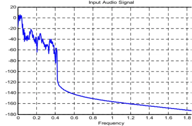
We consider an audio file (.wav file) as the input source instead of a multi-tone frequency signal. The input audio signal, whose frequency response can be seen in Fig.3, with a total of ‘39922’ samples has a sample frequency of 8 kHz. The audio file reads “The discrete Fourier transform of a re-evalued signal is conjugated symmetric”. The sampling frequency of 8 kHz means the highest frequency component is of 4kHz. The objective is to send amplitude modulated waveform into the KZK model and observe the demodulated output at a particular distance [3].

The audio file with an of 4kHz if modulated with a carrier of 5kHz would result in an output signal

with a spectrum of 9kHz. However the 9 kHz is not in the ultrasonic range and remains audible. If this audible modulated signal is passed into the air channel, it will lead to more audible harmonics which translates into distortion. Therefore, we have to upsample the message to a higher rate.

0 0.2 0.4 0.6 0.8 1 1.2 1.4 1.6 1.8 2

x 10⁴ -180

-160 -140 -120 -100 -80 -60 -40 -20 0 20

Frequency

Power Spectrum Magnitude (dB)

Input Audio Signal

Fig. 3 Input Audio Signal

The range of acceptable carrier frequencies is constrained by the message bandwidth. The original message must be upsampled by an integer factor U to ensure that there is no aliasing. To avoid aliasing near DC, we need the carrier frequency _{} _{to be} greater than_{}. The highest frequency possible

in a SSB or DSB signal is then

_{}  _{}  _{}_. _since _the simulations must be carried out digitally, this implies that the overall sampling rate, _{}_{, must be} greater than _{}_.

Now we increase the sampling frequency to 40 kHz.

With a carrier frequency, Fc of 15.9 kHz and a sampling frequency of 40 kHz, the audio signal is square rooted to compensate for distortion and amplitude modulated.

The amplitude modulated signal is passed into the channel, the KZK model. The KZK model will be explained in a subsequent chapter .With a source radius of .15 meters, the Rayleigh distance determines that farfield starts approximately at a distance of 3.20 meters. The amplitude modulation was done with a

(6)

modulation index of 0.7. This modulated signal passed through air, due to the inherent nonlinear properties of air, automatically demodulates and produces the audio output at a certain distance, of 3.7 meters, at the farfield.

0 0.2 0.4 0.6 0.8 1 1.2 1.4 1.6 1.8 2

x 10⁴ -140

-120 -100 -80 -60 -40 -20 0 20 40

Frequency

Modulated Signal

Fig. 4. Amplitude modulated signal

0 0.2 0.4 0.6 0.8 1 1.2 1.4 1.6 1.8 2

x 10⁴ -180

-160 -140 -120 -100 -80 -60 -40 -20 0 20

Frequency

Demodulated data

Original Signal Demodulated data

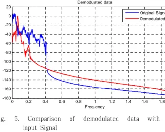
Fig. 5. Comparison of demodulated data with input Signal

From Fig.4, it is plain obvious to see that there exists certain frequency components in the audible range. If there exists frequency components in the audible range, passing this signal through the channel will only generate more harmonics which will lead to a greater level of distortion. In Fig.5 it can be seen that as the demodulated data takes shape, it varies more from the original audio file as evident in the plot.

Therefore, we need to choose a higher carrier frequency.

To begin with, we need to increase the sampling frequency of the audio signal in order to reduce

distortion. Therefore the audio signal was upsampled by an integer factor, U of 10. After upsampling, the audio signal has a sampling frequency  of 80kHz as can be seen in Fig.6. This audio signal is then amplitude modulated with a carrier signal of 35.9 kHz.

The amplitude modulated signal does not have a frequency component in the audible range as evident in Fig.7. For a source radius considered to be of 0.15 meters, the farfield distance is determined to begin at a distance of 7.6 meters.

0 0.5 1 1.5 2 2.5 3 3.5 4

x 10⁴ -200

-150 -100 -50 0 50

Frequency

Upsampled signal

Fig. 6. Upsampled audio signal

0 0.5 1 1.5 2 2.5 3 3.5 4

x 10⁴ -160

-140 -120 -100 -80 -60 -40 -20 0 20 40

Frequency

AM upsampled signal

Fig. 7. Amplitude modulated signal

After the upsampled AM signal is passed through the ‘air channel’, and the demodulated data is obtained, as seen in Fig.8, we calculate the Power spectral density (PSD) of the output data. The PSD of the output signal is low due to the high distortion levels that exist in the demodulated data.

Ⅳ. Conclusion

(7)

This work was supported by Defense Acquisition Program Administration and Agency for Defense Development under the contract UD070054AD

저자 소개 이 종 현(정회원)

∙1985년 한양대학교 전자공학과 공학 사

∙1987년 Michigan Technological University 공학석사

∙2002년 한국과학기술원 전기 및 전자 공학과 공학박사

∙1990년~1995년 학국전자통신연구원 선임연구원

∙2000년~2002년 (주) KM Telecom 연구소장

∙2003년 3월~2006년 1월 서경대학교 전자공학과 전임강사

∙2006년 3월 ~ 현재 제주대학교 해양과학대학 해양시스템공 학과 조교수

<주관심분야 : 통계학적 신호처리, 적응 배열 시스템, 수중통 신, 이동통신 시스템, 디지털 TV, UWB 무선전송기술>

Mano Samuel(준회원)

∙2006년 Karunya Institute of Technology and sciences Deemed University 공학사

∙2009년 제주대학교 해양시스템공학과 공학석사

∙2009년 ~ 현재 (주)알고코리아 .

In this paper, parametric array for audio applications is analyzed by numerical modeling and analytical approximation. A time domain finite difference code that accurately solves the KZK nonlinear parabolic wave equation is used to predict the response of the parametric array. The time domain code relates the source size and the carrier frequency to the audible signal response including the output level and beamwidth. In considering the implementation issues for audio applications of the parametric array, the emphasis is given to the frequency response and distortion. Specifically we use the time domain code to find out the optimal parameters that will help produce the parametric array with highest achievable output in terms of the average power within the demodulated signal. Parameters such as primary input frequency and sampling frequency are demonstrated through the numerical simulation.

참 고 문 헌

[1] Mark F.Hamilton and David T.Blackstock,

"Non-linear Acoustics", Academic press, Chestnut Hill, MA. 1998, pp 233-259.

[2] Y.S.Lee, "Numerical simulation of the KZK equation for pulsed finite amplitude sound beams in Thermoviscous fluids". PhD dissertation, The University of Texas at Austin, December 1933.

[3] Masahide Yoneyama and Jun-ichiroh Fujimoto,

"The audio spotlight: An application of nonlinear interaction of sound waves to a new type of loudspeaker design". J.Acoust.Soc.Am, Vol 73, No5, May 1983.

(8)

이 재 일(정회원)

∙2009년 제주대학교 해양산업공학전공 이학사

∙2009년 ~ 현재 : 제주대학교 해양시스 템공학과 석사과정

<주관심분야 : 수중통신, 수중음향, 디 지털 신호처리>

김 원 호(정회원)

∙1984년 단국대학교 전기공학과 학사

∙1993년 부경대학교 전자통신공학과 석사

∙2003년 부경대학교 음향진동공학과 박사

∙1984년 ~ 현재 국방과학연구소 음향센서연구팀 선임연구원

<주관심분야 : 센서 음장 해석, 측정 기법, 수중 음향>

배 진 호(정회원)