New Bubble Size Distribution Model for Cryogenic High-speed Cavitating Flow

New Bubble Size Distribution Model for Cryogenic High-speed Cavitating Flow

Yutaka ITO, Kazuhiro TOMITAKA, Takao NAGASAKI Tokyo Institute of Technology

4259-G3-33, Nagatsuta-cho, Midori-ku, Yokohama, 226-8502, JAPAN [email protected]

Keywords: cavitation, numerical simulation, cryogen, bubble size distribution model Abstract

A Bubble size distribution model has been developed for the numerical simulation of cryogenic high-speed cavitating flow of the turbo-pumps in the liquid fuel rocket engine. The new model is based on the previous one proposed by the authors, in which the bubble number density was solved as a function of bubble size at each grid point of the calculation domain by means of Eulerian framework with respect to the bubble size coordinate. In the previous model, the growth/decay of bubbles due to pressure difference between bubble and liquid was solved exactly based on Rayleigh-Plesset equation. However, the unsteady heat transfer between liquid and bubble, which controls the evaporation/condensation rate, was approximated by a theoretical solution of unsteady heat conduction under a constant temperature difference. In the present study, the unsteady temperature field in the liquid around a bubble is also solved exactly in order to establish an accurate and efficient numerical simulation code for cavitating flows. The growth/decay of a single bubble and growth of bubbles with nucleation were successfully simulated by the proposed model.

1. Introduction 1.1 Cavitation in a cryogenic turbopump

Flagship rockets of each country employ cryogenic LOX/LH2 engines which are superior in controllability, thrust and specific impulse. Its turbopumps are required both to operate at a high rotating speed for small size and high pressure output and to be low NPSH for a light fuel tank. Then, it is almost inevitable that cavitation occurs at the turbopumps. As a countermeasure against cavitation, an inducer impeller is set upstream of radial/axial main impellers of the turbopumps. At heavy load operation, however, unsteady cavitation occurs on the inducer impeller and suction performance becomes unstable[1]. Furthermore, cryogenic cavitation has larger thermodynamic effect than water one[2].

Therefore, cavitation of the turbopumps is very complex. Because it is difficult to predict and control cavitation theoretically[3]/ numerically[4], the turbopump is empirically designed based on visible[1]

and/or trial[5] tests. There is a possibility that the turbopump can be optimized and improved on by the progress of prediction methods.

Hence high accuracy numerical code is desired for easy optimizing, easy improving on, and reducing the

number of trial manufacturing and experiments.

Analyses on cavitation as a basis for developing the code have been proposed by a lot of researchers^[6,7]. Numerical simulation on an inducer by using LES has also been reported by Fujii et al. ^[8] In this report, a simplified homogeneous flow model^[9], which assumes that void fraction changes in proportion to the degree of super saturation, was employed as a cavitation model in contrast to the LES model for the accurate simulation of turbulent flow. Results on qualitative tendency such as tip cavitation was obtained, but qualitative results such as discharge pressure didn’t agree satisfactorily with experimental results. It seems that the imbalance between the simplified cavitation model and exact LES calculation causes insufficient quantitative accuracy. Therefore it is very important to develop a detailed model of cryogenic cavitation in a high speed turbopump.

1.2 Numerical cavitation model for design of a cryogenic turbopump

To build up a numerical model, it is important to manage both strict modeling of cavitation and reasonable computational time applicable for design.

With attention to these points, modeling policies are indicated below.

Gas phase disperses inside liquid phase in a turbopump because of a high speed flow, so the size of each dispersed gas phase is the order of μm to mm, and each shape approaches to spherical. Therefore, a cavitation flow in a turbopump is regarded as a bubbly flow, in other words, gas phase is assumed to be a cloud of spherical bubbles and liquid phase is assumed as a continuum containing bubbles.

In process of bubble growth/decay, Matsumoto et al. reported that incondensable gas plays an important role on bubble phenomena just before collapse[10].

There is a little helium as incondensable gas in a cryogenic turbopump, however, a main purpose of the present study is to evaluate the pump performance, not to analyze microscopic phenomena like erosion.

Therefore, incondensable gas is neglected and each bubble is made of pure vapor due to micro size.

In regard to calculation models for the growth/decay of a vapor bubble, the inertia control model and the heat transfer control model are representable. In the former model, the bubble surface temperature is assumed to be equal to that of surrounding liquid, and the change of bubble radius is calculated based on Rayleigh-Plesset equation. In the latter model, the liquid pressure at the bubble surface is assumed to be equal to that of liquid far from

bubble, and the bubble growth is rate controlled by phase change determined by heat transfer in the liquid.

The former model is valid when the bubble growth/decay is very rapid even if phase change occurs, and the latter is valid when the bubble growth/decay is very slow. In the present model, both mechanisms are incorporated rigorously in order to deal with various bubble behaviors such as bubble oscillation with phase change.

Heterogeneous bubble nucleation model, which is that bubble nuclei are generated in relation to the degree of super saturation, is employed as the nucleation of cavitation bubble.

It is important to take into account the slip velocity between bubbles and their surrounding liquid because bubbles move in a variable pressure field with external force like centrifugal force. Slip velocity depends on the bubble size, so it is necessary to distinguish bubbles with different sizes between the small bubble just after nucleation and the large bubble well grown. Therefore, bubble size distribution model^[11], whereby bubbles are distinguished based on their mass, is employed. The advection velocities and growth/decay rates of bubbles with size distribution are computed by the model.

In this paper, the above numerical model for cavitation was constructed, and it was applied to growth/decay of cryogenic cavitation bubbles in a liquid at various conditions of super saturation and subcool to verify the usefulness of the model.

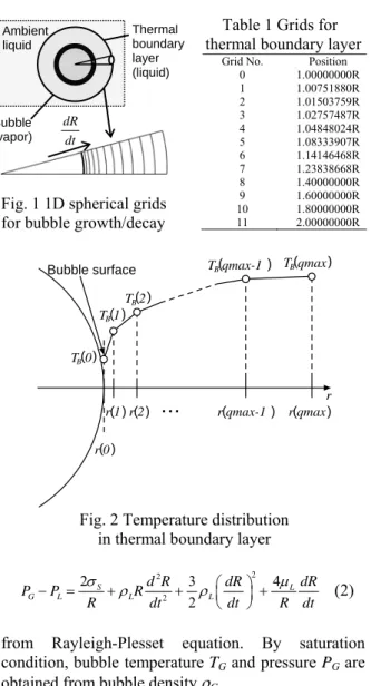
2. Bubble growth/decay in a stationary liquid Bubble radius is calculated by Rayleigh-Plesset equation taking into account the changes of bubble mass and bubble surface temperature due to phase change. Temperature field of liquid phase in the thermal boundary layer around the bubble is calculated simultaneously to determine the phase- change rate and bubble surface temperature. Because the thermal boundary layer varies due to bubble oscillation, spherical numerical grids are laid on thermal boundary layer to solve the temperature distribution.

2.1 Basic equation for bubble growth/decay

One-dimensional spherical coordinate system on a bubble is considered as shown in Fig. 1. r is distance in radial direction, r=0 is at the center of a bubble, r=R is at the surface of a bubble, and r=Rout is the outer boundary of calculation domain. Because the temperature variation occurs mainly in the region r<2R in the case of steady heat conduction around a sphere^[12], Rout is set at 2R. Evaporation/condensation rate for a bubble is calculated by temperature gradient at the bubble surface as follows,

( )

4 2

G L B

surface

w t γ πR k dT dr L

∂ ∂ = = (1)

Here w denotes mass of vapor bubble, L latent heat of vaporization, and TB liquid phase temperature

around the bubble. Bubble growth rate, dR/dt, is governed by

Table 1 Grids for thermal boundary layer

Fig. 1 1D spherical grids for bubble growth/decay

r 0

r 1 r 2 ・・・ r qmax-1 r qmax T 0

T 1 T 2

T qmax-1 T qmax Bubble surface

r

B B

B

B B

( ) ( )

( )

( ) ( )

( )

( ) ( ) ( ) ( )

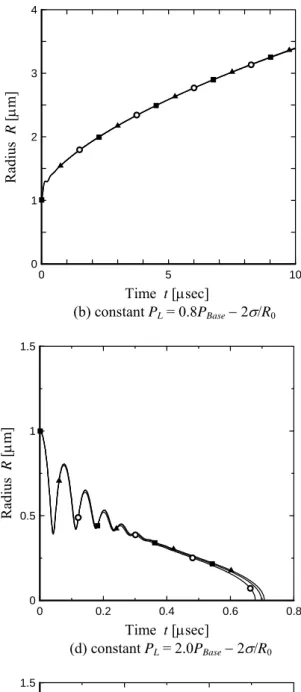
Fig. 2 Temperature distribution in thermal boundary layer

2 2 2

2 3 4

2

S L

G L L L

d R dR dR

P P R

R dt dt R dt

σ ρ ρ ^{⎛ ⎞} μ

− = + + ⎜⎝ ⎟⎠ + (2)

from Rayleigh-Plesset equation. By saturation condition, bubble temperature TG and pressure PG are obtained from bubble density ρ_G.

ρG=3w/(4πR³) (3)

TG=Tsat(ρ_G) (4)

PG=Psat(ρ_G) (5)

Local radial velocity c at r is derived from the surface velocity c|surface.

( )

{ }

2 2 4 2 2 2

surface G L

c=c R r = dR dt−γ π ρR R r (6) Temperature distribution TB is calculated by Lagrangian differential equation on the system moving at local speed c.

2 2

1

B L B

L L

DT k d dT

Dt ⁼ ρCp r dr^⎛⎜⎝r dr ^⎞⎟⎠ (7)

2.2 Analytical method for bubble growth/decay Firstly, the mass rate of phase change, γG, is calculated by using spatial 2nd order discretized form of eq. (1).

Grid No. Position 0 1.00000000R 1 1.00751880R 2 1.01503759R 3 1.02757487R 4 1.04848024R 5 1.08333907R 6 1.14146468R 7 1.23838668R 8 1.40000000R 9 1.60000000R 10 1.80000000R 11 2.00000000R dR

dt Bubble (vapor)

Thermal boundary layer (liquid) Ambient

liquid

( )² [ ¹{ ²( ^{1 2})} ( )

4 ^{old old} 2

G R kL L TB

γ = π −Δ Δ Δ + Δ (8)

( ^{1 2}) ( ^{1 2})TB^old( ) (1 2 ^{1 2}){ ¹( ^{1 2})}TG^old]

+ Δ + Δ Δ Δ − Δ + Δ Δ Δ + Δ

where, TB(q), r(q) are values at grid point q, where q is index of grid as shown in Fig. 2. Grid interval Δ1=r^old(1) −R^old, and Δ2=r^old(2) −r^old(1). Positive γGmeans evaporation.

The bubble mass at the new time step, w, is obtained by explicit time marching of eq. (1) with time interval ΔtR.

old

G R

w=w + Δγ t (9)

where superscript, old, denotes previous time step.

Bubble radius, R, is calculated from dR/dt by the following procedure based on eq. (2).

nth stage: (dR/dt)ⁿ=(dR/dt)^old+f(R^an,(dR/dt)^an,bⁿΔt_R)

Rⁿ=R^old+ (dR/dt)ⁿ bⁿΔt_R (10) where

( )

(

)

f R dR dt b tΔ = P −P − σ R (11)

( )

{ }

3 2ρL dR dt ^an 4μL R^an dR dt ^an⎤b tn R ρLR^an

− − ⎦ Δ

Applying Jameson’s factors, an=(old, 1, 2, 3), bn=(1/3, 4/15, 5/9, 1) for n=1 to 4, eq. (10) becomes 4 stages Runge-Kutta method with temporal 2nd order accuracy. New values of ρG, TG and PG are obtained by eqs. (3) to (5). TB is calculated by implicit time marching using spatial 2nd order and temporal 1st order discretized equation derived from eq. (7).

( ) ( )

( )

2 2

2

B Bold L B B

R L L q q

T q T q k dT d T

t Cp r q dr dr

Δ ρ

⎧ ⎫

− = ⎨⎩ ⎛⎜⎝ ⎞⎟⎠ +⎛⎜⎝ ⎞⎟⎠ ⎬⎭ (dTB/dr)q={g11TB(q−1)+g₁₂TB(q)+g13TB(q+1)} (12) (d²TB/dr²)q={g21TB(q−1)+g22TB(q)+g23TB(q+1)}

g11=−Δ₂/{Δ₁(Δ₁+Δ₂)}, g12=(Δ₂−Δ₁)/(Δ₁Δ₂), g13=Δ1/{Δ2(Δ1+Δ2)}, g21=2/{Δ1(Δ1+Δ2)}, g22=−2/(Δ₁Δ₂), g23=2/{Δ₂(Δ₁+Δ₂)}

Δ₁=r(q) − r(q−1), Δ₂=r(q) − r(q+1) Then, the following equation is obtained.

a(q)TB(q−1)+b(q)TB(q)+c(q)TB(q−1)=d(q) (13) a(q)= −k_L/(ρ_LCpL){g11/r(q)+g12},

b(q)=1/Δt_R−k_L/(ρLCpL){g12/r(q)+g22}

c(q)= −kL/(ρLCpL){g13/r(q)+g23}, d(q)=TB^old(q)/ΔtR

The above equation is organized into a matrix form.

( ) ( ) ( ) ( ) ( )

( ) ( )

( )( ) ( )

( )

1 0 0

1 1 1 1

2 2 2

1 1

1 0

B B B

max max

B max

T

a b c T

a b T

b q c q

T q

⎛ ⎞

⎛ ⎞

⎜ ⎟

⎜ ⎟

⎜ ⎟

⎜ ⎟

⎜ ⎟

⎜ ⎟

⎜ ⎟

⎜ − − ⎟⎜ ⎟

⎜ ⎟⎜ ⎟

⎝ ⎠⎝ ⎠

O M

M

( ) ( ) ( ) ( )

(T dG^{, 1 ,}d ^{2 ,}d ^{3 , ,}d qmax ^{1 ,}TL)^transpose

= L − (14)

Under TB(0)=TG and TB(qmax)=TL, TB is solved by diagonalizing the factor’s matrix. Due to implicit method, limitation of time interval can be ignored for TB calculation. However, limitation of time interval is imposed due to bubble oscillation, and the time

interval is determined by using natural frequency for vapor bubble by Prosperetti^[13] as follows.

( )

1

R na R

t f C

Δ = (15)

( ) ( ³ )

1 2 3 2

na p equ sat S L equ

f = π κ R P − σ ρ R

where, the constant, CR, are set to 20, and the equivalent bubble radius Requ is given by a representative bubble size of the calculation. Index κP

approaches to specific heat ratio γ_SHR for high frequency. In case of dtB/dr|surface>0 and large Δt_R, some bubbles unphysically become super critical bubbles, TG>critical temperature Tc, and dissolve into liquid. So, temperature change ΔT_G during Δt_R is limited to be smaller than 10%Tc.

Δt_R=γ_G,LimitL/{4πR²kL(dTB/dr)|surface} (16) γ_G,Limit=4πR³{ρ_sat(TG+0.1Tc)−ρG^old}/3

Because TB is calculated by Lagrangian framework based on eq. (7), the new value of TB for each old grid point corresponds to the temperature at the distance c(q)Δt_R away from position of old grid point.

Therefore TB at the new grid points, as indicated in Table 2, is interpolated by cubic spline approximation.

2.3 Result of a single bubble growth/decay in a stationary liquid at constant pressure

The growth/decay behavior of a bubble in liquid nitrogen is shown in Fig. 3. A bubble with R0=10⁻⁶m and TG0=0.75Tc is put into the liquid at t=0. Liquid temperature and pressure far from the bubble are assumed to be constant with respect to time. Liquid pressure is set to balanced pressure with initial bubble pressure and surface tension of the bubble. Liquid temperature is parametrically changed from superheat to subcool conditions. Three kind of numerical grids for the thermal boundary layer are employed as followings.

Type1:　1=0.0010R and 1000 grid points (uniform), Type2:　1=0.0075R and 133 grid points (uniform), Type3:　1=0.0075R and 11 grid points (non-uniform, see Table 1).

Thermal boundary layer with thickness 10 %R0 and linear temperature profile is assumed as an initial condition in order to give the same initial temperature profile independent of grid interval. Because results by type 1 and type2 agree well in all cases, it is verified that results by type 1 are rigorous.

Calculation load, i.e. computational time, by type 3 is smaller by a factor of 90 compared with by type 1.

The difference between the results by type 3 and rigorous ones by type1 is small (5% error at maximum), so it is verified that type 3 grids is enough to obtain bubble behaviors.

Figure 4 shows results under the same condition as Fig. 3, except that liquid temperature is set to equilibrium temperature with initial bubble temperature and liquid pressure is parametrically changed from 50% to 1000% saturation pressure of equilibrium temperature. In case of superheat

^{0 5 10}

0 2 4 6 8

^{0 5 10}

0 1 2 3

Time t [μsec] Time t [μsec]

(a) constant TL = TBase + 10 (b) constant TL = TBase + 2

^{00 5 10}

1 2

^{00 5 10}

1 2

Time t [μsec] Time t [μsec]

(c) constant TL = TBase + 0.5 (d) constant TL = TBase

^{00 5 10 15}

0.5 1 1.5

^{00 2 4}

0.5 1 1.5

Time t [μsec] Time t [μsec]

(e) constant TL = TBase − 0.5 (f) constant T_L = TBase − 2 Fig. 3 Comparison of results by using various numerical grids in case of constant TL, PL

LN2, TBase = 0.75Tc, PBase = Psat(TBase), Δt=10⁻¹², PL=PBase − 2σ/R₀, TG0 = TBase, PG0 = PBase

Radius R [μm] Radius R [μm]

Radius R [μm] Radius R [μm]

Radius R [μm] Radius R [μm]

1000 grids 133 grids

11 grids(Inequality)

^{0 5 10}

0 5 10

^{0 5 10}

0 1 2 3 4

Time t [μsec] Time t [μsec]

(a) constant PL = 0.5PBase − 2σ/R₀ (b) constant PL = 0.8PBase − 2σ/R₀

^{00 5 10}

1 2

^{00 0.2 0.4 0.6 0.8}

0.5 1 1.5

Time t [μsec] Time t [μsec]

(c) constant PL = PBase − 2σ/R₀ (d) constant PL = 2.0PBase − 2σ/R₀

^{00 0.005 0.01 0.015 0.02}

0.5 1 1.5

^{00 0.004 0.008 0.012}

0.5 1 1.5

Time t [μsec] Time t [μsec]

(e) constant PL = 5.0PBase − 2σ/R0 (f) constant PL = 10.0PBase − 2σ/R0

Fig. 4 Comparison of results by using various numerical grids in case of constant TL, PL

LN2, TBase = 0.75Tc, PBase = Psat(TBase), Δt=10⁻¹², TL=TBase, TG0 = TBase, PG0 = PBase

Radius R [μm]

Radius R [μm] Radius R [μm] Radius R [μm]

Radius R [μm] Radius R [μm]

1000 grids

133 grids

11 grids(Inequality)

N_G

0 Bubble size (mass of a bubble) s [kg]

(a) Bubble size distribution in some region NG(slight,l) NG(sheavy,l)

0 Bubble size (mass of a bubble) s [kg]

(b) Simple classification of NG on s NG(slight,l) NG(sheavy,l)

0 Bubble size (mass of a bubble) s [kg]

(c) More accurate classification of NG on s Fig. 5 Bubble size distribution model

conditions, i.e. smaller liquid pressure, the initial bubble growth is in condition of inertia control. In some cases oscillation occurs in the early period as seen in Fig. 4(b) by the following reason: Due to the initial rapid growth, evaporation is insufficient to support bubble growth, so the bubble pressure reduces and the bubble shrinks momentarily because inertia wins pressure difference between the bubble and liquid. After that the bubble pressure recovers and the bubble regrows. The amplitude gradually decreases and the bubble behavior shifts to moderate growth controlled by heat transfer. On the other hand in case of subcool conditions, the bubble just after insertion shrinks in condition of inertia control. Due to the rapid decrease of bubble radius, condensation is insufficient to keep bubble decay, so the bubble pressure rises and the bubble rebounds momentarily because inertia wins pressure difference between the bubble and liquid.

After that the bubble pressure reduces and the bubble shrinks again. The amplitude of oscillation gradually decreases and the bubble behavior shifts to moderate decay controlled by heat transfer. Because the agreement between type 3 and the rigorous one (type1) is almost satisfactory, it is verified that the present numerical model is appropriate to simulate bubble behavior even in the case of growth/decay with oscillation.

3. Bubble growth/decay by using BSD model Bubble size distribution model whereby bubbles are distinguished based on their mass, advection velocity are calculated, and growth/decay rates are computed using Eulerian framework, is employed.

3.1 Basic equation for bubble growth/decay by BSD

In order to employ bubble mass w as the measure of bubble size for Eulerian framework, an independent

variable s is is introduced.

s=4π ρR³ _G 3 (17)

Namely, bubble mass axis s is defined in addition to the spatial axes x, y, z. It should be noted that the definition of s is the same as w, but w is dependent variable. An example of bubble distribution in a certain volume is shown in Fig. 5(a) by probability density function NG of bubble number density nG. as a function of s. Basic equations can be written as conservative equations of NG.

( ₀)

( )

G G G G

N t N γ s Π δ s w

∂ ∂ + ∂ ∂ = − (18)

(sN_G) t (sN_{G G}γ ) s sΠ δ_G (s w₀) N_{G G}γ

∂ ∂ + ∂ ∂ = − + (19)

(RN_G) t (RN_{G G}γ ) s R₀Π δ_G (s w₀)

∂ ∂ + ∂ ∂ = − (20)

(

)

∂ & ∂ + ∂ & ∂ = & − (21) (T N_{B G}) t (T N_{B G G}γ ) s T_LΠ δ_G (s w₀)

∂ ∂ + ∂ ∂ = − (22)

In these equations, Π_G denotes nucleation rate (number of generated bubbles due to nucleation per unit volume per unit time), w0 mass of one nucleated bubble, and γ_G evaporation (condensation for negative value) rate per one bubble of size s. Because the mass of one bubble increase with time due to the evaporation, bubbles move at speed γG in s direction.

In the same way, sN_G, R(s), R&(s) and T_B(r, s) also move in s direction.

3.2 Discretization of basic equation with respect to the bubble mass axis for BSD

NG is discretized with respect to coordinate s, and conservative values nG,l , mG,l are defined for the discretized region (sub region) in the s coordinate.

, , ,

heavy l

light l s

G l G

n ≡

∫

( )

, ,

, , , ,

heavy l

light l s

G l G average l G l l G l

s

m ≡

∫

Conservation equation for nG,l , mG,l are derived from eqs. (18)(19).

[ ] ,^,

, s^{heavy l}_{light l} ,

G l G G s G G l

n t N γ Π Φ

∂ ∂ + = − (25)

[ ] _,^,

, ^{heavy l} 0 , , ,

light l s

G l G G s G G l G l G l

m t sN γ wΠ Ψ n γ

∂ ∂ + = − + (26)

In order to solve new values of nG,l , mG,l by using eqs. (25)(26), the profile of NG in the sub region must be assumed, as shown in Fig. 5(b)(c), because the boundary values of each sub section are required in the 2nd term of left-hand side of eqs. (25)(26). It should be noted that the hatched area of the l th sub region in Fig. 5(b)(c) corresponds to nG,l based on eq.

(23). A uniform profile shown in Fig. 5(b) is simple, however, the profile is determined uniquely only by nG,l obtained from eq. (25), and mG,l cannot satisfies Probability function of nG NG [1/m3 kg]

Probability function of nG NG [1/m3 kg]

Probability function of nG NG [1/m3 kg]

l−1 class

l class

l+1 class

eqs. (24) and (26) simultaneously. On the other hand, by using a linear profile shown in Fig. 5(c), the profile is determined uniquely to satisfy eqs. (23)-(26).

Therefore a linear profile is employed. The linear distribution has 3 patterns. Pattern 1 is the case of (slight,l+2sheavy,l)/3≤wl, Pattern 2 is the case of (2slight,l+sheavy,l)/3≤wl≤(slight,l+2sheavy,l)/3 and Pattern 3 is the case of wl≤(slight,l+2sheavy,l)/3.

Pattern 1: s_min=3w_l−2s_{heavy l,},s_max=s_{heavy l,}

( )

( )

( ) { }

, , ,

,

, , ,

2 3

0

2 3( )

light l heavy l l heavy l

Gw light l

Gw heavy l G l heavy l l

s s w s

N s

N s n s w

+ ≤ <

=

= −

(27)

Pattern 2: s_min=s_{light l,},s_max=s_{heavy l,},Δ =s s_{heavy l,} −s_{light l,}

( ) ( )

( )

( )

, , , ,

2

, , , ,

2

, , , ,

2 3 2 3

2 (3 2 )

2 (2 3 )

light l heavy l l light l heavy l

G light l G l l light l heavy l

G heavy l G l heavy l light l l

s s w s s

N s n w s s s

N s n s s w s

+ < < +

= − − Δ

= + − Δ

(28)

Pattern 3: s_min=s_{light l,},s_max=3w_l−2s_{light l,}

( )

( ) { }

( )

, , ,

, , ,

,

2 3

2 3( )

0

light l l light l heavy l Gw light l G l l light l Gw heavy l

s w s s

N s n w s

N s

< ≤ +

= −

=

(29)

In case of growth and wl≤(slight,l+2sheavy,l)/3, distribution is pattern 3 and there is no flux into class l+1 because of NG(sheavy,l)=0. After bubble growth, in case that wl becomes larger than (slight,l+2sheavy,l)/3, distribution is pattern 2 and flux into class l+1 exists because NG(sheavy,l) gets a positive value. Namely, bubbles grow into heavier class only in case of patterns 1 and 2, and bubbles decay into lighter class only in case of patterns 2 and 3. This function prevents numerical diffusion on interclass growth/decay of bubbles.

3.3 Calculation method for bubble growth/decay by BSD

Figure 6 shows a flowchart of bubble growth/decay calculation by using BSD.

Firstly, time intervals Δt_F, Δt_R, Δt_S, Δt_P are determined, where Δt_F is for the flow calculations, Δt_R for the calculations of Rayleigh-Plesset eq. and thermal boundary layer at each class at each grid, Δt_S for the interclass calculations in s direction (time marching of bubble size distribution) at each grid, Δt_P for the liquid temperature and pressure calculations at each grid. They have relationship of Δt_F≥Δt_P≥Δt_S≥ Δt_R. Δt_F is decided by CFL condition. Δt_P is decided by Eq. (15) and CR=5. Δt_S is decided by the following stability condition for Eq. (26).

, , 1

l G l S heavy l

w +γ Δ ≤t s + , w^l−γ^{G l,} Δ ≥t^S s^{light l, 1}− (30)

Because γG,l is unknown before calculation shown in chapter 2, conceivable maximum γ_G,l is assumed and Δt_S is estimated. γG,l is proportional to dTB/dr|surface

and Rl squared as shown in Eq. (1). In case of decay, because both dTB/dr|surface and Rl are decreasing during ΔtS, initial γG,l can be regarded as maximum.

(

)

S l light l G l

t w s ₋ γ

Δ ≤ − (31)

Fig. 6 Flowchart for BSD

In case of growth, both dTB/dr|surface and Rl are increasing during Δt_S. Conceivable maximum Rmax,l is

33s_{heavy l}, 1₊ 4πρ_G at bubble mass sheavy,l+1 from stable condition of Eq. (20). dTB/dr|surface becomes larger because of increasing Rl , but it becomes smaller because of thermal diffusion. For γ_Gmax,l calculation, it is enough to consider dTB/dr|surface only in case of increasing temperature gradient. New grid interval

r′0,l

Δ is calculated from Δr_0,l =r1,l−r_0,l by using Eq. (6) wherein the evaporation term in the right hand side is ignored.

r′0,l=R0,l+dRl/dt ΔtS≤Rmax,l (32) r′1,l=R0,l+Δr_0,l+dRl/dt {R_0,l² /(R_0,l+Δr_0,l)²}ΔtS (33)

Calculate temporal change of liquid conservative values, α’Lρ’L, α’Lρ’Lu’L, α’Lρ’Lv’L, α’Lρ’Lw’L, α’Lρ’Le’L, bubble variables, nG,l, m G,l, Rl, R^•l, TB,q,l due to convection

loopP loopS

Start calculation by using values at time n as initial value Calculate time intervals ΔtF, ΔtP, ΔtS, ΔtR for loopG, loopP, loopS, loopR. Calculate the number of calculation χP, χS, χR for loopP, loopS, loopR.

Focus on each grid (only 1 grid in the present paper)

Calculate Rl, R^•l, TB,q,l after Δt’R by using calculation procedure in chapter 2 with Rl, R^• l, TB,q,l as initial conditions and TL, PL as boundary conditions. Then calculate γG,l

Focus on each class l

number of cal.<χR

Distinguish nucleation and calculate R0l, ΠG,l in case of nucleation

Values at time n+1 are fixed Yes

Calculate ρL by αLρL, αL and calculate eL by αLρLeL, αLρL

Calculate αG,l by Rl, nG,l and calculate αL=1-∑αG,l

Calculate TL by eL and PL by ρL, TL using physical properties loopR

number of cal.<χS

Yes

All girds No

Yes

loopG

Do interclass calculation as shown in sections 3.1 and 3.2 by results of loopR, γG,l, R0l, ΠG,l. Calculate nG,l, mG,l, Rl, R^•l, TB,q,l after Δt’S

By results of loopS, calculate ΦG,l, ΨG,l during Δt’P

Calculate nG,l, mG,l, Rl, R^•l, TB,q,l after Δt’P by results of loopS and convection

Calculate α’Lρ’L, α’Lρ’Lu’L, α’Lρ’Lv’L, α’Lρ’Lw’L, α’Lρ’Le’L after Δt’P by results of loopS and convection

number of cal.<χP

r′0,l

Δ =Δr_0,l−dR_l/dtΔr_0,l(2R0,l+Δr_0,l) Δt_S/(R0,l+Δr_0,l)² (34) Because dRl/dt≤(Rmax,l−R0,l)/ΔtS is obtained from Eq. (32), eq. (34) is rewritten as

r′0,l

Δ /Δr_0,l ≤1−(R_max,l−R_0,l)(2R0,l+Δr_0,l)/(R0,l+Δr_0,l)² (35) Temperature gradient is inversely proportional to grid interval as indicated by eq. (1), so γ_Gmax,l is given

by γGmax,l/γG,l=(Rmax,l−R_0,l)²/(Δr′_0,l/Δr_0,l) (36)

From eqs.(30) and (36), the stability condition of Δt_S is expressed by

( )( )

( )

, 0, 0, 0,

, 1 0, 0, 2

, , 2

0,

1 ^{max l l} 2 ^{l l}

heavy l l l l

S

G l max l

l

R R R r

s w R r

t R

R γ

+

⎛ − − + Δ ⎞

⎜ ⎟

− ⎝ + Δ ⎠

Δ ≤ ⎛⎜⎝ ⎞⎟⎠

(37)

Δt’_P, Δt’_S, Δt’_R employed in the practical calculation are decided as

Integer: χP=ceiling(ΔtF/ΔtP), Δt’P=ΔtF/χP (38) Integer: χ_S=ceiling(Δt’_P/Δt_S), Δt’_S=Δt’_P/χ_S (39) Integer: χ_R=ceiling(Δt’_S/Δt_R), Δt’_R=Δt’_S/χ_R (40)

0 Mass s [kg] 10⁻¹⁴ t =0.00 [μsec]

t =0.25 [μsec]

t =0.50 [μsec]

t =2.00 [μsec]

t =10.00 [μsec]

Fig. 7 Continuous nucleation into the constant temperature and pressure liquid by BSD LN2, TBase = 0.75Tc, PBase = Psat(TBase), Δt=10⁻¹⁰ TL=TBase, TG0 = TBase, PL = PBase − 2σ/R₀, PG0 = PBase

s1=10⁻¹⁶ (si=10^(i−49)/3) x 9 classes, R0 = 0.5μm

-0.1 0 0.1 0.2 0.3 0.4 0.5

0 400 800 1200

0 0.1 0.2 0.3 0.4 0.5

time t [μsec]

(a) liquid nitrogen

-0.1 0 0 0.1 0.2 0.3 0.4 0.5

500 1000 1500

0 0.1 0.2 0.3 0.4 0.5

(b) liquid oxygen

^{-0.1 0 0.1 0.2 0.3 0.4 0.5}

0 100 200 300 400 500

0 0.1 0.2 0.3 0.4 0.5

(c) liquid hydrogen

-0.025 0 0.025 0.05 0.075 0.1

0 1000 2000 3000 4000 5000 6000

0 0.1 0.2 0.3 0.4 0.5

(d) water

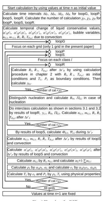
Fig. 8 Temporal change of Rl, PL after bubble insertion at t = 0 into liquid at constant volume by BSD LN2, TBase =0.75Tc, PBase=Psat(TBase), TL0=TG0=TBase, PL0=PBase−2σ/R0, PG0=PBase, Δt=10⁻¹¹[sec]

s₁=10⁻¹⁸ (s_i=10^(i−55)/3) x 7 classes, R₀=0.5μm x 10¹⁵個/m³ x (once at first)

Pressure P [kPa] Pressure P [kPa] Pressure P [kPa] Pressure P [kPa] Radius R [μm] Radius R [μm] Radius R [μm] Radius R [μm]

nG,l [1/m3] αG,l [-] 1x10^-9 0 5x10³ 0