Long Term Chlorophyll-a Prediction Based on the Rise in Sea-Water Temperature Using the Eco-Hydrodynamic
Model in the Yellow Sea
Chul-hui Kwoun*··Min-sun Kwon*··In-Sung Han**··Young-sang Seo**·· Jae-Dong Hwang**··Hoon Kang*··Nam-do Lee*
Land & Ocean Environment Co.,Ltd., Suwon, 443-470, Korea*
Ministry for Food, Agriculture, Forestry & Fisheries, Busan, 619-705, Korea**
(Manuscript received 4 March 2010; accepted 6 July 2010)
생태-유체역학 모델을 이용한 해수 수온 상승에 따른 황해 Chlorophyll- a의 장기 변화 예측
권철휘*·권민선*·한인성**·서영상**·황재동**·강훈*·이남도*
(주)국토해양환경기술단*, 국립수산과학원**
(2010년 3월 4일 접수, 2010년 7월 6일 승인)
Abstract
수산·해양환경적 측면에서 중요한 위치에 있는 황해(Yellow Sea)의 해양 생태계 변화과정에 대 한 체계적이고 심층적인 연구을 위하여 기후 변화와 관련된 생태 및 환경변화에 대한 황해 해역의 반응성 연구가 필요한 실정이다. 본 연구는 황해해역에서 수온 상승에 따른 클로로필의 변화를 살펴 보고, 지구온난화가 해양환경과 생태계에 미칠 영향을 예측하고자 하였다. 황해해역에서 해수유동 모델의 결과를 기초 입력자료로 활용하여 클로로필과 상호작용을 하는 육상유입부하량, 저질 영양 염용출량 및 생물학적 파라메타 등을 입력하여 현재상태를 재현하였다. 우리나라 주변 해수의 온도 가 지난 10년간 약 0.75℃ 상승했다고 가정하였을 때, 본 실험에서는 수온이 선형적으로 연간 0.075℃ 씩 상승한다고 가정하여 10년 후까지의 Chlorophyll-a 농도 변화를 예측하였다. 예측 결 과, 연구해역의 중앙부에서는 전체적으로 농도가 높아지고, 우리나라 연안해역에서 Chlorophyll-a 의 농도가 낮아지는 것으로 예측되었다. 본 연구의 결과를 기초로하여 10년 이상의 장기적인 예측실 험을 한다면 기후변화가 황해해역의 생태계 변화에 미치는 영향을 파악할 수 있을 것으로 기대된다.
주요어 : Yellow Sea, Climate Change, Sea Surface Temperature, Ecological Model, Chlorophyll-a
Corresponding Author: Chul-Hui Kwoun, Land Ocean Environment Co.,Ltd., D-1301, Digitalempire I., #980-3, Yeontong-dong, Yeongtong- gu, Suwon-si, Gyeonggido, Korea Tel: 82-31-221-7812~3 Fax: 82-31-221-7801 E-mail: [email protected] 연구논문
I. Introduction
Currently there are numerous instances of nat- ural disasters all across the globe, such as typhoons, hails, and draughts. Many researches and studies point to climate changes as the main cause behind such calamities. Although climate changes take place over a long period of time, the recent report from the UN Intergovernmental Panel on Climate Change (IPCC) predicts that global warming caused by human activities will be speeding up, along with its impacts on Earth.
Global warming has a great impact on the Earth’s environmental systems, including the atmosphere, the ocean, and the land. Due to its proximity with the atmosphere, the ocean wit- nesses a rise in sea level resulting from the heat expansion caused by a rise in sea surface temper- ature, and this serves as a threat to those living in coastal regions. The rise in sea surface temper- ature also has a direct impact on the marine ecosystem and is expected to gradually influence the fishery resources; yet predictions and the nec- essary countermeasures against such phenome- non is severely lacking at the moment.
Due to the large inflow of fresh water from land, the Yellow Sea boasts an abundance in nutritive salts that play an important role in the reproduction of organisms. Thanks to this it is considered an important territory for diverse types of fish, for it provides a suitable environ- ment for growth and habitation to phytoplank- tons, zooplanktons and the fish that feed on these organisms. Geographically speaking, the Yellow Sea is made up of a wide continental shelf adjacent to Korea and its neighbors, and it has complex environmental characteristics due to the various sea currents and water masses that come into contact within its boundaries, such as
Kuroshio, Taiwan Warm Current, Yellow Sea Warm Current, Korean Coastal Waters, Changjiang Diluted Waters, China Coastal Waters, and Yellow Sea Bottom Bold Water(Naimie et al., 2001; Zhang & Weng, 1996).
Although nothing definite has been found out regarding the movement of sea currents taking place at the continental shelf, recently studies are being conducted regarding water mass distribu- tion and flow fields with the use of satellite data and such. Meanwhile, it is well known that Kuroshio and Taiwan Warm Current are flowing into Yellow Sea at the continental shelf break, but the existence of YSWC(Yellow Sea Warm Current) remains unclear. Because the flow field of such seawater is closely related to substance distribution, its simulation is mandatory for gath- ering information when predicting substance dis- tribution caused by changes in the ocean envi- ronment. On the other hand, in order to figure out the changes that take place within the ocean ecosystem as a response to outer environmental changes, detailed information regarding physical factors as well as the prediction of changes in land inflow load, changes in water temperature and salinity caused by the changes in fresh water inflow, and the long-term biogeochemical trans- formation, is needed. In this regard, there is a lack of systematic and comprehensive researches on the changes taking place in the Yellow Sea’s ecosystem, and studies on the sea’s reactivity in the face of various eco-environmental changes caused by global warming and other phenomena are needed.
Therefore, focusing on the Yellow Sea, this study aims to provide basic data that can be used to come up with countermeasures against changes in the ocean environment caused by climate
changes, by predicting the impacts of the rise in sea surface temperature on the ocean environ- ment and ecosystem using the ecosystem model.
II. Method
In the study the eco-hydrodynamic model was used for the simulation of Yellow Sea’s tides, water temperature and other factors related to the ecosystem (Kremer & Nixon, 1978; Nakata et al., 1983). This model is made up of multi-level hydrodynamic model (COSMOS), used for the sea water flow simulation, and the ecological model (EUTRP 2), used for the water quality simulation.
1. Hydrodynamic modeling
The basic equation for fluid kinematics consists of equation of motion, continuity equation, free surface (tide level) equation, chlorinity budget (chlorinity diffusion equation), heat budget(ther- mal diffusion equation) and the equation of state regarding ocean density. These can be expressed as follows:
1) Equation of motion of the x-direction
= _ (u2) _ (uv) _ (uw) + fov (1)
_g _
∫
x 0 dz′_+ (Nx ) + (Ny ) + (Nz )
2) Equation of motion of the y-direction
= _ (uv) _ (v2) _ (vw) + fou (2)
_g _
∫
z 0 dz′_+ (Nx ) + (Ny ) + (Nz )
3) Continuity equation
+ + = 0 (3)
4) Free surface(tide level) equation
= (
∫
_Hx udz) _ (∫
_Hx vdz) (4)5) Heat budget equation(thermal diffusion equation)
= _ (uT) _ (vT) _ (wT) (5)
+ (kx ) + (ky ) + (kz )
6) Equation of state
r = r(Cl, T) (6)
Here u, v, w represent the velocity compo- nents (cm/sec) of the X-, Y-, and Z-directions.
The ocean density r was calculated using the Knudsen equation. Each parameter used in the equations have the following meaning:
z: The distance between the mean sea level and free surface level(cm)
H: The distance between the mean sea level and the ocean floor(cm)
r: Fluid density(g/cm3) f0: Coriolis parameter(sec-1) g: Gravity acceleration(cm/sec2) Pa: Atmospheric pressure(g/cm·sec2) T: Water temperature(˚C)
Cl: Chlorinity
Nx, Ny, Nz: Kinematic eddy viscosity of the x-, y-, and z- directions(cm2/sec)
Kx, Ky, Kz: Kinematic eddy diffusion coefficient of the x-, y-, and z-directions (cm2/sec)
kx, ky, kz: Thermal diffusivity of the x-, y-, and z- directions (cm2/sec)
In order to give Kuroshio and the Taiwan sea currents full consideration, the model area was widened to include the northern parts of Taiwan and parts of Kyushu in Japan. The grid consisted of 147 lines in the x-direction and 202 lines in the y-direction. The size of each grid was 1/12˚ in both directions. The water layers were divided
∂T
∂z
∂
∂z
∂T
∂y
∂
∂y
∂T
∂x
∂
∂x
∂
∂z
∂
∂y
∂
∂x
∂T
∂t
∂
∂y
_∂
∂x
∂x
∂t
∂w
∂z
∂v
∂y
∂u
∂x
∂v
∂z
∂
∂z
∂v
∂y
∂
∂y
∂v
∂x
∂
∂x
∂Pa
∂y 1 r
∂r
∂y g r
∂x
∂y
∂
∂z
∂
∂y
∂
∂x
∂v
∂t
∂u
∂z
∂
∂z
∂u
∂y
∂
∂y
∂u
∂x
∂
∂x
∂Pa
∂x 1 r
∂r
∂x g r
∂x
∂x
∂
∂z
∂
∂y
∂
∂x
∂u
∂t
into 6 layers(Level 1: 0~20m, Level 2: 20~40m, Level 3: 40~60m, Level 4: 60~80m, Level 5:
80~100m, Level 6: deeper than 100m).
The input data related to external conditions, water temperature, salinity and such used in this study was obtained through research. The bot-
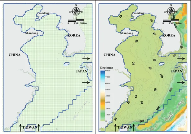
tom friction coefficient used was 0.0022, the opti- mal value for deep seas which is considered to provide stability to values. The horizontal kine- matic eddy diffusion coefficient and the horizon- tal kinematic eddy viscosity used were 1.0×106 cm2/sec, like Kim et al.(1999). The vertical diffu- Fig. 1. Grid map and bathymetric map of the target sea area
Table 1. Initial input data for hydrodynamic model
Grid information Applied Arakawa C-Grid, Dx=Dy=approxi. 9.26Km(147×202) Level 1: 0~20m, 2: 20~40m, 3: 40~60m, 4: 60~80m, 5: 80~100m, 6: 100m below
Total simulation time 1year
Calculation step 120 sec
Initial values water temp. and sal. temp. : 8.1~25.9˚C, sal. : 31.9~32.9 Water temp. and sal. at open boundary temp. : 22.3~26.0˚C, sal. : 31.9~34.9 Horizontal viscosity and diffusion coefficient Level 1~6 : 1.0E6(cm2/s)
Vertical diffusion coefficient Level 1~6 : 0.1(cm2/s)
Bottom friction coefficient 0.0022
Wind Time series during 1 year Using NIMR/KMA WIND WAVES 2008 DB
Ocean current 3sv~24sv(1sv=106m3/s)
Parameters and forcing Input values
sion coefficient was 0.1 cm2/sec fro layer 1 to layer 6. For water temperature the initial value, which was based on the summer season, was consistently entered for all areas, and the initial values of the water temperatures of the Taiwan sea currents and Kuroshio were entered for each open boundaries. For winds, the time series data spanning one year regarding changing locations was entered using the 「NIMR/KMA WIND WAVES 2008 DB」. In order to take the sea cur- rents into account, a simulation was carried out in which the load volumes(3sv, 24sv(1vs=
106m3/s)) of the Taiwan currents and Kuroshio at the southern and eastern open boundaries were entered. For Kuroshio this was repeated a few more times by adjusting the load volume accord- ing to the depth of water at each open boundary.
2. Ecological modeling
Regarding the phytoplankton component in the ecosystem model, it was necessary to take into account the average clusters of single species in the sea area. In sea areas where succession of species was apparent it was necessary to observe these multiple groups in terms of how they build up nutrients inside their bodies and how they react to temperature, light, and nutritive salts.
The model was simplified as much as possible since there were many indefinite factors in select- ing the biological parameter related to competi-
tion among species. Taking all these into account, the change in the number of phytoplanktons P(mg C/m3) according to time changes can be expressed as equation (7).
= photosynthetic growth-Extracellular
release-respiration-grazing by (7) zooplanktons-natural mortality-sinking
The equation that shows the change over time in concentration B, which represents the existing amount of a component at a random spot in the sea area, can be expressed as follows:
= _ u _ v _w (8)
+
[
Kx]
+[
Ky]
+[
Kz]
+
Here,
x, y, z: Coordinate parameters t: Time
u, v, w: Velocity components of the X-, Y-, and Z- directions
Kx, Ky, Kz: Kinematic eddy diffusion coefficient of the x-, y-, and z-directions
B: Existing amount of a component(or its concentration) dB/dt: Amount of change(per time unit) in the component caused by all biological and chemical processes
Because the above-mentioned diffusion equa- tion calculates the substance movements caused by the flow, the ecosystem model is related to
∂B
∂t
∂B
∂z
∂
∂z
∂B
∂y
∂
∂y
∂B
∂x
∂
∂x
∂B
∂z
∂B
∂y
∂B
∂x
∂B
∂t dP dt
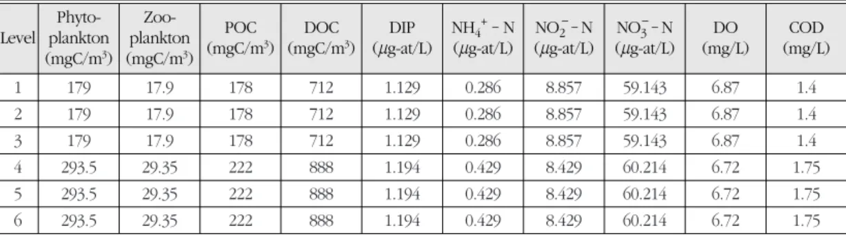
Table 2. Initial input data for ecosystem model
Level Phyto- Zoo- POC DOC DIP NH4+ _N NO2__ N NO3__ N DO COD
plankton plankton (mgC/m3) (mgC/m3) (mg-at/L) (mg-at/L) (mg-at/L) (mg-at/L) (mg/L) (mg/L) (mgC/m3) (mgC/m3)
1 179 17.9 178 712 1.129 0.286 8.857 59.143 6.87 1.4
2 179 17.9 178 712 1.129 0.286 8.857 59.143 6.87 1.4
3 179 17.9 178 712 1.129 0.286 8.857 59.143 6.87 1.4
4 293.5 29.35 222 888 1.194 0.429 8.429 60.214 6.72 1.75
5 293.5 29.35 222 888 1.194 0.429 8.429 60.214 6.72 1.75
6 293.5 29.35 222 888 1.194 0.429 8.429 60.214 6.72 1.75
Phyto- Zoo-
POC DOC DIP NH4+ _N NO2__ N NO3__ N DO COD
Level plankton plankton
(mgC/m3) (mgC/m3) (mg-at/L) (mg-at/L) (mg-at/L) (mg-at/L) (mg/L) (mg/L) (mgC/m3) (mgC/m3)
the 3-dimesional hydrodynamic model. When the velocity components(u, v, w), which are calculat- ed from the simulation of the flow model, are entered into the ecosystem model, the existing amount of each component is predicted accord- ing to changes in time and space. The initial input values for the ecosystem model were cho- sen based on the data gathered from research and from on-site surveys of the target sea areas, and they took into account the spatial distribu- tion factor, as it can be seen in tables 2 and 3.
The variables used in the flow model were used for the horizontal and vertical diffusion variables of substances. Regarding fresh water sources that pass from land to the target sea area through rivers and streams, only the Han river, Yellow
river and Yangtze river were entered. Lee’s(2005) data was used for the ejected amount of sedi- ment nutritive salts.
III. Results and Discussion
Using the influx data provided by Lee and Chao(2003) as a reference for input data, the amount of inflow and outflow was set as 3sv for the Taiwan Warm Currents and as 24sv for Kuroshio warm currents, in order to make the calculation more convenient. Also, because the target sea area was a typical monsoon area influ- enced by northwesterly winds during winter and southeasterly winds during summer, the data from January to December of 2008 was entered in monthly time-series using variable wind sys- tem(Wxt, Wyt) 「NIMR/KMA WIND WAVES 2008 DB」, which changes according to time and space. The direction of the wind was altered as east-west and north-south components before
Table 4. Biological parameters
Phytoplankton
Maximum growth rate day-1 0.54 exp (0.0633T)
Half saturation constants for nutrient mg/L Phosphate 0.3
Nitrogen 3.0
Respiration rate day-1 0.01 exp(0.0524T)
Sinking rate of living cells m/day 0.15
Rate of nature mortality, a4 day-1 0.054 exp(0.0693T)
Zooplankton
Maximum grazing rate, a3 day-1 0.18 exp(0.0693T)
Ivlev constant, l (mg C/m3)-1 0.01
Feeding threshold, P* mg C/m3 75
Energy expenditure in grazing activity, n - 30% of the daily carbon ration
Assimilation efficiency, m % 70.0
Rate of natural mortality, a5 day-1 0.054 exp(0.0693T)
Organic carbon
Mineralization rate of detritus, a6 day-1 0.01 exp(0.0693T)
Sinking rate of detritus, WPOC m/day 0.4
Mineralization rate of dissolved organic matter, a7 day-1 0.004 exp (0.0693T)
Parameter definition Unit Value
Table 3. Amount of fresh water inflow (Kim, 1999; Kim et al., 1999)
1 (Han) 109,700,000
2 (Yellow) 114,900,000
3 (Yangtze) 691,200,000
Sources (NO) Mean discharge (ton/day)
being entered. On a slightly different note, as much as 80,000m3/s of inflow comes into the tar- get sea area from China’s Yangtze river during summer. In order to simulate the impacts caused by such inflow of fresh water, the summertime influx from the Han river, Yellow river and Yangtze river were entered. In this case a Sponge Boundary was set up over as many as 3 grids, and the amount of flow as well as the velocity were also given in order to induce stable results.
Meanwhile, focusing on the currents, wind fields and the inflow of fresh water at the same time, in the test the water temperature was changed in the following 4 stages: 1 year later, 2 years later, 5 years later, 10 years later. The results derived from the hydrodynamics in summer were entered as the basic flow field of the ecosystem model. It was assumed that the water temperature would increase linearly at the same value. Comparing the data on average temperature in the East
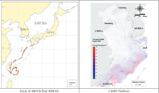
China Sea from 1989-1998 with that of the year 2008, provided by National Fisheries Research and Development Institute, it was found that the sea surface temperature had risen by approxi- mately 0.75˚C during the past ten years. Based on this it was assumed that the water temperature of the target sea area would rise by 0.075˚C every year. Because it was difficult to verify the average seawater circulation over a long period of time that exceeds the tide cycle in such a wide area, the verification was carried out carefully using data from previous studies instead (fig. 2). As a result the simulation of Kuroshio, Taiwan Warm Currents and other nearby sea currents in the East China Sea was quite successful. Also, based on the results from the seawater circulation analy- sis the present concentration distribution of Chlorophyll-a was carefully verified through a comparison with satellite data(MODIS, NASA) (fig. 3). In this case the data consisted of the aver-
Fig. 2. Comparison between the ARGOS Current Chart (Korea Hydrographic and Oceanographic Administration: KHOA) and the results from the Hydrodynamic Model
Track of ARGOS float (KHOA) CASE0 (Surface)
age concentration level of Chlorophyll-a measured from the surface to a point 4m deep in the water
according to turbidity, whereas the Chlorophyll-a concentration calculated in the model was that Fig. 3. Comparison of the model’s results with MODIS imagery of the surface Chlorophyll-a
Surface Chlorophyll-a in July 2009(MODIS, NASA)
Surface Chlorophyll-a in July 2007(MODIS, NASA) Surface Chlorophyll-a in July 2008(MODIS, NASA)
CASE0 (Surface)
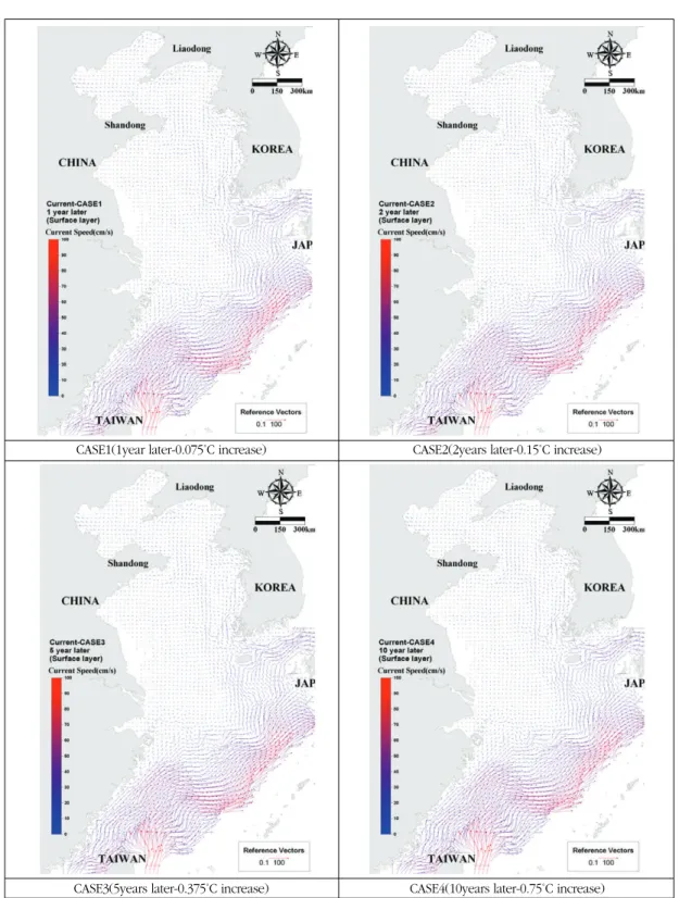
Fig. 4. Changes in seawater circulation according to the rise in water temperature : After 0.075˚C(CASE1), 0.15˚C(CASE2), 0.375˚C(CASE3), 0.75˚C(CASE4) increase in temperature
CASE3(5years later-0.375˚C increase)
CASE1(1year later-0.075˚C increase) CASE2(2years later-0.15˚C increase)
CASE4(10years later-0.75˚C increase)
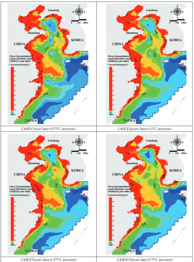
Fig. 5. Changes in Chlorophyll-a concentration of Layer 1(surface) according to the rise in water temperature : After 0.075˚C (CASE1), 0.15˚C(CASE2), 0.375˚C(CASE3), 0.75˚C(CASE4) increase in temperature
CASE3(5years later-0.375˚C increase)
CASE1(1year later-0.075˚C increase) CASE2(2years later-0.15˚C increase)
CASE4(10years later-0.75˚C increase)
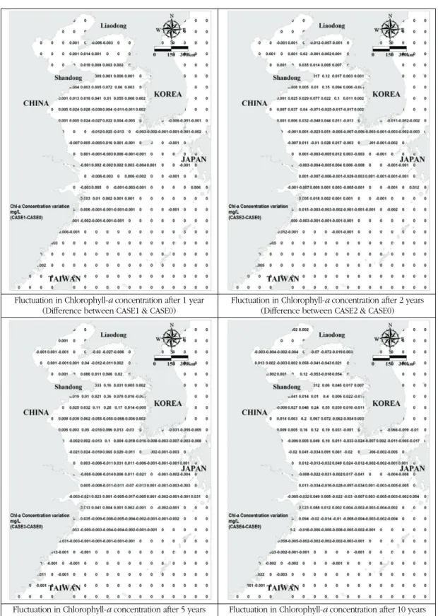
Fig. 6. Fluctuations in Chlorophyll-a concentration according to the rise in water temperature Fluctuation in Chlorophyll-a concentration after 1 year
(Difference between CASE1 & CASE0)
Fluctuation in Chlorophyll-a concentration after 2 years (Difference between CASE2 & CASE0)
Fluctuation in Chlorophyll-a concentration after 10 years (Difference between CASE4 & CASE0) Fluctuation in Chlorophyll-a concentration after 5 years
(Difference between CASE3 & CASE0)
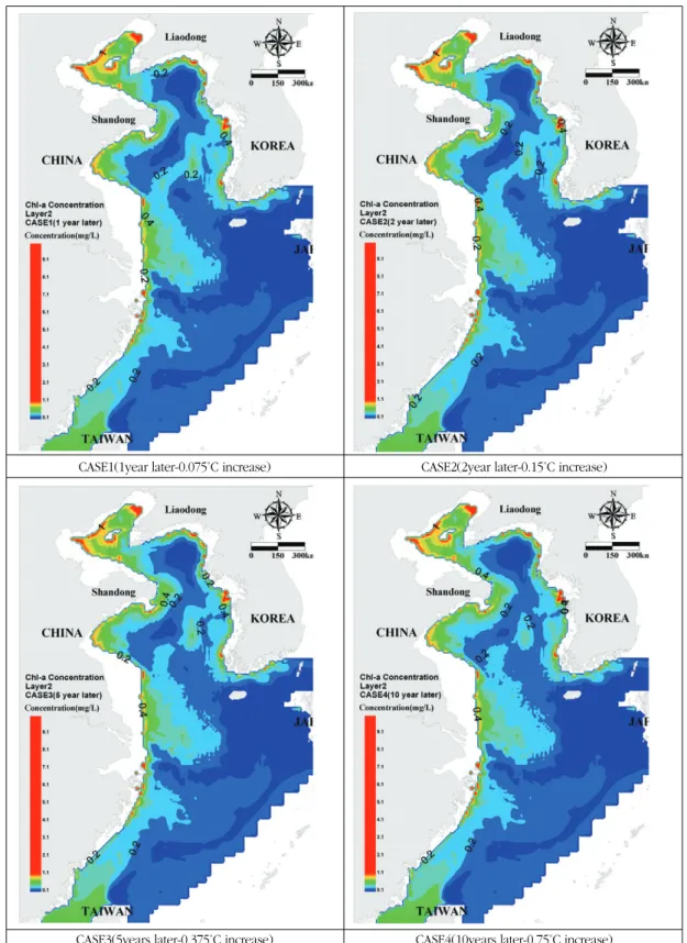
Fig. 7. Changes in Chlorophyll-a concentration in Layer 2 according to the rise in water temperature : After 0.075˚C(CASE1), 0.15˚C(CASE2), 0.375˚C(CASE3), 0.75˚C(CASE4) increase in temperature
CASE3(5years later-0.375˚C increase)
CASE1(1year later-0.075˚C increase) CASE2(2year later-0.15˚C increase)
CASE4(10years later-0.75˚C increase)
measured at a depth of 10m. The Chlorophyll-a concentration distribution found on the surface was low in the Taiwan and Kuroshio warm cur- rents, due to the formation of oligotrophic water masses. The concentration level was high along the coasts and lower in the ocean. The close resemblance between the satellite images showing the average concentration distribution of Chlorophyll-a in July of 2007, 2008, and 2009 and the Chlorophyll-a distribution pattern derived from the model points to a relatively successful simulation of the current conditions.
Meanwhile, there weren’t any noticeable differ- ences in the seawater circulation between the pre- sent and 10 years later (fig. 4), despite the hypo- thetical rise of 0.75˚C in temperature. An analysis, based on the sea circulation results, of the changes in Chlorophyll-a caused by the rise in water temperature showed that 10 years later the concentration level of Chlorophyll-a would rise by approximately 0.55mg/L. The results also con- firmed that the overall concentration would increase. Since the circulation pattern displayed by the Taiwan and Kuroshio currents is not affected greatly by the rise in temperature, it can be assumed that the center of the Yellow Sea is not influenced greatly by the oligotrophic water masses. However, the concentration level mea- sured in the northern parts of the Shandong peninsula and along the Liadong peninsula coasts decreased by as much as 0.05mg/L, and in the Yellow sea it decreased by as much as 0.06mg/L. The Chlorophyll-a concentration decreased also along the coasts, while its varia- tion within the central area of the Yellow Sea ranged between -0.06mg/L~+0.55mg/L, show- ing the greatest fluctuation. This leads to the pre- diction that the ecological changes along the
Korean coasts and within the Yellow Sea will be greater than those along the Chinese coasts and within the East China Sea.
Layer2 represents the Chlorophyll-a concentration at a point 30m deep in the water. In this case, coastal areas shallower than this depth were not included in the calculation of the concentration. Not including the coastal regions shallower than Layer2, the overall distribution pattern of Chlorophyll-a did not differ greatly from that of the surface, although the concentration itself was lower than that detected on the surface. In particular, due to Kuroshio the concentration level was below 0.1mg/L in the southern sea of Korea and the western sea of Japan, whereas it was relatively higher in the East China Sea. Also, unlike on the surface of the water, the Chlorophyll-a concentration did not increase along with the rise in temperature.
IV. Conclusions
Concentrating on Kuroshio and Taiwan Warn Currents found in the Yellow Sea and East China Sea during summer, this study simulated the sea- water circulation while taking into account the variable wind system and influx load of fresh water, and evaluated the changes in Chlorophyll- a caused by the rise in sea surface temperature.
Since a quantitative verification was difficult due to time and spatial restrictions, the movement of seawater was simulated and the trace of ARGO was meticulously verified, which resulted in a realistic calculation of the currents. Also, when the distribution of Chlorophyll-a concentration detected during summertime was simulated using the Ecosystem model, the results were quite similar to the average Chlorophyll-a distrib- ution pattern detected by satellites in July from
2007 to 2009. There was no discernible change in sea water circulation with the rise of the sea sur- face temperature. However, after 10 years the amount of chlorophyll-a increased by 0.55mg/L in the central area of the Yellow Sea, and the overall concentration level increased in the target sea area. In particular, in Korea the concentration decreased along the coasts, while its variation within the central area of the Yellow Sea ranged between -0.06mg/L~+0.55mg/L, showing the greatest fluctuation. This leads to the prediction that the ecological changes along the Korean coasts and within the Yellow Sea will be greater than those along the Chinese coasts and within the East China Sea. Although in this study the chlorophyll-a concentration did not display any drastic increase after the rise in the sea surface temperature, a more long-term simulation is expected to clarify the change patterns and yield reliable predictions about ecological changes.
Acknowledgements
This study was carried out as a part of the
“Study on the Changes in the Fishery Environment Caused by Climate Change” (RP-2010-ME-025), a research led by the Fishery and Ocean Information Division at the National Fisheries Research &
Development Institute.
Bibliography
Journal of the Korean Society for Marine Environmental Engineering, 2, 63-73. (in Korean)
Kim, D. M., 1999, The eutrophication modeling in the Yellow Sea using an ecosystem model, PhD Dissertation, Department of
Environmental Engineering, Pukyong National University, 143p. (in Korean) Kim, G. S., Kim, D. M., and Park, C. K., 1999, A
Rough Estimation of Environmental Capacity in the Yellow Sea using a Numerical Hydrodynamic Model, Journal of the Korean Society for Marine Environmental Engineering, 2, 63-73. (in Korean)
Kremer, J. N. and Nixon, S. W., 1978, A coastal marine ecosystem simulation and analysis, Springer-Verlag, 217.
Lee, D. I., Cho, H. S., Yun Y. H., Choi Y. C., and Lee, J. H., 2005, Summer environmental evaluation of water and sediment quality in the South Sea and East China Sea, Journal of Korean Society for Marine Environmental Engineering, 8, 83-99. (in Korean)
Lee, H.-J. and S.-Y. Chao, 2003. A climatological description of circulation in and around the East China Sea. Deep-Sea Research II 50, 1065-1084.
Naimie, C. K., Blain, C. A., and Lynch, D. R., 2001, Seasonal mean circulation in the Yellow Sea - a model-generated climatology, Continental Shelf Research, 21, 667-695.
Nakata, K., Horiguchi, F., Taguchi, K., and Setoguchi, Y., 1983. Three dimensional tidal current simulation in Oppa Bay, Bulletin of the National Research Institute for Pollution and Resources, 12, 17-36. (in Japanese)
Zhang, Q. L. and Weng, X. C., 1996, Analysis of water masses in the south Yellow Sea in Spring, The Yellow Sea, 2, 74-82.
최종원고채택 10. 07. 12