Hyper-Parameter in Hidden Markov Random Field

Hyper-Parameter in Hidden Markov Random Field

Johan Lim

· Donghyeon Yu

· Kyungsuk Pyun

1

Department of Statistics, Seoul National University

2

Department of Statistics, Seoul National University;

Samsung Electronics Company

(Received April 2010; accepted November 2010)

Abstract

Hidden Markov random field(HMRF) is one of the most common model for image segmentation which is an important preprocessing in many imaging devices. The HMRF has unknown hyper-parameters on Markov random field to be estimated in segmenting testing images. However, in practice, due to computational com- plexity, it is often assumed to be a fixed constant. In this paper, we numerically show that the segmentation results very depending on the fixed hyper-parameter, and, if the parameter is misspecified, they further de- pend on the choice of the class-labelling algorithm. In contrast, the HMRF with estimated hyper-parameter provides consistent segmentation results regardless of the choice of class labelling and the estimation method.

Thus, we recommend practitioners estimate the hyper-parameter even though it is computationally complex.

Keywords: Hidden Markov random field, hyper-parameter, image segmentation.

1. Introduction

Segmentation is a process which divides an image into several homogeneous regions, whereas clas- sification matches an unknown image with a known image in the database. Despite their apparent difference, classifiers are often used for segmenting an image with the name of context-based clas- sifier.

A context-based classifier partitions the whole image into many sub-blocks and classifies each sub- block into one of the classes in the database. In doing so, a difficulty arises in obtaining smooth boundaries, which is often a trait of the true segmentation. To obtain smooth boundaries, hidden Markov models(HMM) have often been proposed, in which the spatial coherence between sub-blocks is modelled by the Markovian random field (Geman and Geman, 1984; Besag, 1986; Li and Gray, 1999; Li et al., 1999). The Ising model or the Potts model are popularly used depending on the number of classes in the true segmentation.

Suppose the observed image has n × n pixels and is denoted as X = {X

, 1 ≤ i ≤ n, 1 ≤ j ≤ n}.

Let Z

∈ {0, 1} be the true class assigned to the image X

and Z = {Z

, 1 ≤ i ≤ n, 1 ≤ j ≤ n}

Johan Lim’s research was supported by Basic Science Research Program through the National Research Foundation of Korea(NRF) funded by Ministry of Education, Science and Technology(No. 2010-0011448).

1Corresponding author: Associate Professor, Department of Statistics, College of Natural Sciences Seoul National University, Daehak-dong, Gwanak-gu, Seoul 151-747, Korea. E-mail: [email protected]

denotes the true hidden segmentation corresponding to X . A common assumption for the true segmentation Z is a symmetric nearest neighborhood(SNN) Ising model with α:

P ( Z = Z) = 1 Ψ(α) exp

 

 α · ∑

∀(i,j)∼(k,l)

V (Z

, Z

)

 

 , (1.1)

where Ψ(α) is a normalizing constant, and V (Z

, Z

) = 1 if Z

= Z

, and 0 otherwise. Given Z, the observed image Z is from conditionally independent distributions, in which P (X

= x |Z

= 1) = f

(x) and P (X

= x |Z

= 0) = f

(x). Here, the distributions f

(x) and f

(x) are estimated from training data set and assumed to be known in segmentation procedure.

A main goal of image segmentation is to find the true class label Z from observed image X . The most common estimate of Z, given known hyper-parameter α, in previous literature is the maximum a posteriori(MAP) estimate which is defined by

Z b

= argmax

P (Z = Z|X = X) .

In practice, the hyper-parameter α associated with the Markov random field is unknown a priori and training data to estimate it are rarely available. Thus, it must be estimated directly from the given image data, whose maximum likelihood estimator(MLE) is the solution to

∑

∀(i,j)∼(k,l)

E {V (Z

, Z

) |X } = ∑

∀(i,j)∼(k,l)

E {V (Z

, Z

) } , (1.2)

where the expectation in right-hand side(RHS) is analytically known, but that in left-hand side(LHS) is approximated using various methods and is hard to compute. Due to this reason, we assume that α is known and fixed it as a subjectively chosen constant (Won and Gray, 2004).

In this paper, we demonstrate that it is better to estimate hyper-parameter than to fix it in all three image segmentation method - Gibbs Sampling, simulated annealing(SA) and iterative conditional mode(ICM).

2. Alternating Procedure to Jointly Estimate Class Labels and Hyper-parameter

In this section, we assume the observed image X is binary and Z is from the bond percolation model for notational simplicity. Given Z, the observed image X is from conditionally independent Bernoulli distributions, in which P (X

= 1 |Z

= 1) = p

and P (X

= 1 |Z

= 0) = p

. Here, model parameters p

and p

are accurately estimated from training data and are assumed to be known. Further, we rewrite (1.1) as

P (Z = Z) = exp

 

 log ( q

1 − q )

· ∑

∀(i,j)∼(k,l)

V (Z

, Z

)

 

 ,

where q is the probability that any adjacent pixels are independently in equal state.

In this model, the estimating equation (1.2) becomes

n

· q = ∑

∀(i,j)∼(k,l)

E {I (Z

= Z

) |X } , (2.1)

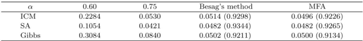
Table 3.1. Misclassification error rate. The numbers in parenthesis are the estimates of α.

α 0.60 0.75 Besag’s method MFA

ICM 0.2284 0.0530 0.0514 (0.9298) 0.0496 (0.9226)

SA 0.1054 0.0421 0.0482 (0.9344) 0.0482 (0.9265)

Gibbs 0.3084 0.0840 0.0502 (0.9211) 0.0500 (0.9134)

As stated before, evaluating E( · |X ) is computationally hard, and various approximations for it has been proposed in previous literature. Besag (1986) uses E {I(Z

= Z

) |X } ≈ I( b Z

= b Z

), where Z b

s are the current MAP estimate of Z

. Second, the mean field approximation(MFA), which is originally designed to approximate derivatives of the partition function, uses E {I(Z

= Z

) |X } ≈ E{I(Z

= Z

)| b Z

, X } (Zhou et al., 1997).

Both approximations utilize the current MAP estimate of Z, for which several Monte Carlo proce- dures are proposed. Geman and Geman (1984), Celeux and Diebolt (1985), and Wei and Tanner (1991) propose to use Gibbs samples of Z. Lavielle and Moulines (1997) use simulated anneal- ing(SA), whereas deterministic annealing is adopted by Ueda and Nakano (1995). Iterative condi- tional mode(ICM) is proposed by Besag (1986). Swendsen and Wang (1987), Diebolt and Ip (1996), Liu (2001) also address the Monte Carlo procedures for the Ising model.

In summary, overall procedure is the alternation between (i) get the MAP class label given cur- rent estimate bα and (ii) update the estimate of α using current MAP of Z. However, due to computational complexity, many authors assume hyper-parameter is a known constant.

3. Examples 3.1. Simulated image

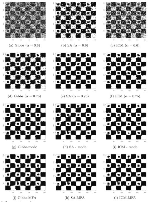
We implement an experiment to show the importance of the hyper-parameter in segmenting an image. The true class labels Z we use is the check-board image presented in Figure 3.1 (a).

The observed image X is generated using symmetric channel P (X

= 1 |Z

= 1) = 0.7 and P (X

= 1 |Z

= 0) = 0.3. We employ three methods (ICM, SA, and Gibbs sampling) to find MAP class labels. We use two methods, Besag’s mode approximation and mean field approximation (MFA) to estimate hyper-parameter α. We also run the cases with fixed α as 0.6 and 0.75. The misclassification rate and parameter estimates for each case we consider are reported in Table 3.1.

The visual segmentation results are reported in Figure 3.1.

The segmentation with an estimated hyper-parameter shows better performance in both misclas- sification error rate and visual segmentation. The results further shows that SA performs well in wider range of fixed parameter α. However, unlike other two class labelling algorithms, the SA re- quires further specification on tempering schedule, for which, in our simulation, a linear tempering is chosen by trial and error. Thus, it is not very surprise that the SA performs better than Gibbs sampling and ICM when α is mis-specified. In both Besag’s method and MFA, the hyper-parameter was chosen as approximately 0.92 regardless of class labelling algorithm. In summary, we find that the hyper-parameters in HMRF is quite important to get better segmentation results.

3.2. Aerial image

In this section, we consider the segmentation of a real noisy binary image.

(a) Gibbs (α = 0.6) (b) SA (α = 0.6) (c) ICM (α = 0.6)

(d) Gibbs (α = 0.75) (e) SA (α = 0.75) (f) ICM (α = 0.75)

(g) Gibbs-mode (h) SA - mode (i) ICM - mode

(j) Gibbs-MFA (k) SA-MFA (l) ICM-MFA

Figure 3.1. Segmentation results

The database we use is composed of six aerial photographs of different locations in the San Francisco

Bay Area. Each photograph is 1024 × 1024 and is a gray-level image with 8 bits per pixel. In each

photo, white represents the manmade class, whereas black represents the natural class. It is paired

with aired with its hand-labelled classified image. These photographs have also been studied by

Aiyer et al. (2005), Li et al. (2000), Pyun et al. (2007) and Pyun et al. (2009). In the analysis, we

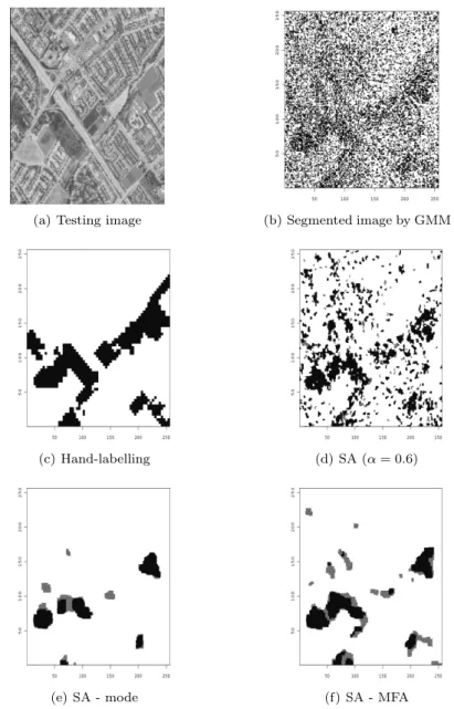
(a) Testing image (b) Segmented image by GMM

(c) Hand-labelling (d) SA (α = 0.6)

(e) SA - mode (f) SA - MFA

Figure 3.2. Segmentation of an aerial image

use 5 photos as training photos and one for testing.

To design computer-based system to measure the spatial correlation in land use, we first segment the

images into manmade and natural area using a block-based classifier. In this paper, we use Gauss

mixture based(GMM) classifier, which divides the image into blocks and is modeled separately using

Gauss mixture model. In the analysis, we use 4 × 4 sub-blocks (256 × 256 sub-blocks in total) and

estimating the Gauss mixture model for manmade and natura regions using 5 training images. The

block processing steps are same with those in Aiyer et al. (2005) and Pyun et al. (2007) and their

details are omitted here. Using the estimate GMMs, we classify each sub-block into the class having

the highest likelihood. The testing image and segmented image by GMM are plotted in the top two panels in Figure 3.2.

We apply the simulated annealing algorithm, which shows the best performance in the simulated data, with several choices of hyper-parameter α. In this example, the segmented result for α = 0.75 is similar to that with estimated τ using MFA, and is not reported here. Again, the segmentation results depend on the choice of α. However, both estimates based on the mode approximation and MFA provide similarly reliable segmentations although the former is slightly smoother than the latter.

4. Conclusion

In this paper, we numerically show that the segmentation results very depending on the pre-specified hyper-parameter in HMRF based image segmentation. On the other hand, the HMRF with es- timated hyper-parameter provides segmentation results which are robust to the choice of class- labelling algorithm as well as the estimation method. In consequence, we recommend practitioners estimate the hyper-parameter although it is rather computationally expensive.

Acknowledgments

We are grateful to the associate editor and two reviewers for their constructive comments.

References

Aiyer, A., Pyun, K., Huang, Y., O ´Brien, D. B. and Gray, R. M. (2005). Lloyd clustering of Gauss mixture models for image compression and classification, Signal Processing: Image Communication, 20, 459–

485.

Besag, J. (1986). On the statistical analysis of dirty pictures, Journal of the Royal Statistical Society-B, 48, 259–302.

Celeux, G. and Diebolt, J. (1985). The SEM algorithm: A probabilisitic teacher algorithm derived from the EM algorithm for the mixture, Computational Statistics Quarterly, 2, 73–82.

Diebolt, J. and Ip, E. H. S. (1996). Stochastic EM: Method and application, In: Gilks W. R., Richardson S. T. and Spiegelhalter D. J., Editors, Markov Chain Monte Carlo in Practice, Chapman & Hall, London.

Geman, S. and Geman, D. (1984). Stochastic relaxation, Gibbs distribution, and the Bayesian restoration of images, IEEE Transaction on Pattern Analysis and Machine Intelligence, 11, 689–691.

Lavielle, M. and Moulines, E. (1997). A simulated annealing version of the EM algorithm for non-Gaussian deconvolution, Statistics and Computing, 7, 229–236.

Li, J. and Gray, R. M. (1999). Image classification based on a multi-resolution two dimensional hidden Markov model, Proceedings International Conference, 1, 348–352.

Li, J., Najmi, A. and Gray, R. M. (1999). Image classification by a two dimensional hidden Markov model, Acoustics, Speech, and Signal Processing, IEEE International Conference, 6, 3313–3316.

Li, J., Najmi, A. and Gray, R. M. (2000). Image classification by a two dimensional hidden Markov model, IEEE-Transaction on Signal Processing, 48, 517–533.

Liu, J. S. (2001). Monte Carlo Strategies in Scientific Computing, Springer-Verlag, Germany.

Pyun, K. S., Lim, J. and Gray, R. M. (2009). A robust hidden Markov Gauss mixture vector quantizer for a noisy source, IEEE-Transaction on Image Processing, 18, 1385–1394.

Pyun, K. S., Lim, J., Won, C. S. and Gray, R. M. (2007). Image segmentation using hidden Markov Gauss mixture model, IEEE-Transaction on Image Processing, 16, 1902–1911.

Swendsen, R. H. and Wang, J. (1987). Nonuniversal critical dynamics in Monte Carlo simulations, Physics Review Letters, 58, 86–88.

Ueda, N. and Nakano, R. (1995). Deterministic annealing variant of the EM algorithm, Neural Information Processing Systems, 7, 545–552.

Wei, G. C. G. and Tanner, M. A. (1991). Applications of multiple imputation to the analysis of censored regression data, Biometrics, 47, 1297–1309.

Won, C. S. and Gray, R. M. (2004). Stochastic Image Processing, Springer, New York.

Zhou, Z., Leahy, R. M. and Qi, J. (1997). Approximate maximum likelihood hyperparameter estimation for Gibbs priors, IEEE Transaction on Image Processing, 6, 844–861.