http://dx.doi.org/10.7840/kics.2015.40.12.2324
충격성 잡음에 강인한 코렌트로피 기반 블라인드 알고리듬의 성능분석
김 남 용
Performance Analysis of Correntropy-Based Blind Algorithms Robust to Impulsive Noise
Namyong Kim
요 약
충격성 잡음하의 블라인드 신호처리 분야에서 최대 상호 코렌트로피 알고리듬 (MCC)이 MSE 기반의 알고리듬 에 비해 우수한 성능을 보인다. 그러나 MCC 알고리듬에 대한 최적 가중치 조건들이나 충격성 잡음에 대한 내성 과 관련된 특성들은 아직 충분히 연구되지 못한 상태이다. 이 논문에서는 MSE기반의 LMS 알고리듬과 비교를 통 해 MCC의 최적 가중치의 성질을 분석하여 MCC 알고리듬의 최적 가중치가 MSE기반의 LMS 알고리듬과 같 다는 보인다. 또한 MCC의 최적 가중치가 충격성 잡음 하에서도 동요 없이 안정을 유지하는 요인이 입력 크기 조 정에 있다는 것을 시뮬레이션을 통해 입증하였다.
Key Words : Cross-correntropy, Random symbols, Impulsive noise, Optimum weight, Magnitude controlled, Equalizer
ABSTRACT
In blind signal processing in impulsive noise environment the maximum cross-correntropy (MCC) algorithm shows superior performance compared to MSE-based algorithms. But optimum weight conditions of MCC algorithm and its properties related with robustness to impulsive noise have not been studied sufficiently. In this paper, through the analysis of the behavior of its optimum weight and the relationship with the MSE-based LMS algorithm, it is shown that the optimum weight of MCC and MSE-based LMS have an equal solution. Also the factor that keeps optimum weight of MCC undisturbed and stable under impulsive noise is proven to be the magnitude controlled input through simulation.
First Author : Division of Electronic, Information and Commun. Eng., Kangwon National Univ., 종신회원
논문번호:KICS2015-09-310, Received September 15, 2015; Revised November 19, 2015; Accepted December 2, 2015
Ⅰ. Introduction
Multipath propagation in wireless channel and impulsive noise from a variety of sources affects the communication systems adversely[1,2]. In the environment with impulsive noise, many signal processing methods based on MSE fail to function
properly because of large instantaneous errors and instability[3].
As an alternative to the MSE criterion, the correntropy criterion similar to auto-correlation has been introduced[3]. The cross-correlation (CC) concept can be expressed with inner products of two different distribution functions constructed by kernel
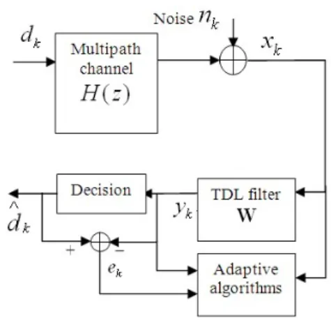
Fig. 1. Base-band communication system and adaptive equalizer structure
density estimation methods with Gaussian kernel
[3,4]
. Through maximization of CC (MCC) with steepest descent method and a set of symbol samples generated randomly at the receiver, the MCC algorithm has been developed for blind channel equalization in the environment of impulsive noise and multipath distortions[5].
One of the drawbacks of MCC algorithm is heavy computational complexity related with summation operations at each iteration time since gradients are calculated based on block processing method. This problem of computational complexity has been significantly reduced in the work [6] by utilizing recursive estimation of the gradient. Though the MCC algorithm has been developed to be better suited to practical situations and problems, analytic research on its optimum solutions and their behavior has not been carried out yet deterring further enhancement of the algorithm.
Ⅱ. MSE Criterion and MCC Algorithm
As depicted in Fig. 1, the baseband model of communication system, the transmitted symbol point dk at time k is distorted by the channel’s multipath fading and added noise nk. For the multipath channel model H(z)=∑hiz−i in z-transform, the equalizer input xk becomes (1)[7].
k i k i
k hd n
x =
∑
− + (1)With the TDL (tapped delay line) equalizer
structure, the input vector
T L k j k k k
k=[x,x−1,...,x−,...,x−+1]
X and weight vector
T k L k j k k
k=[w0,,w1,,..,w,,...,w−1,]
W , the output is expressed
as yk=XTkWk and the error ek is
k T k k k k
k d y d
e = − = −X W (2)
Then the MSE criterion PMSE is defined as a statistical average E[⋅] of squared error ek2.
] [ k2
MSE Ee
P =
] [ 2 ] [ ]
[dk2 kTE Tk k k kTEdk k
E +W XX W − W X
= (3)
Letting the gradient ∂W
∂PMSE
be zero, the optimum weight vector
o
WMSE for MSE criterion can be obtained[8].
] [
] [
k T k
k o k
MSE E
d E
X X
W = X (4)
Inserting this optimum weight WMSEo in the correlation E[ekXk] leads to
0 ] [ ] [ ]
[ek k =Edk k − kE Tk k =
E X X W X X (5)
As a typical algorithm based on the MSE criterion, LMS (least mean square) is to use the instant error power e instead of k2 E[ek2] for practical reasons[7]. Then the gradient of LMS becomes
W
W ∂
−
= ∂
∂
∂ ( )
2
2
k k k
k d y
e e
k k T k k k
k d
eX 2( X W)X
2 =− −
−
= (6)
And
W W
W ∂
⋅∂
−
+ =
2
1 k
k k
μ e =Wk+2μ⋅e Xk k (7)
The optimum weight vector of LMS algorithm
o
WLMS can be obtained as below by letting the gradient ∂W
∂ek2
in (6) be zero.
k T k
k o k
LMS
d X X
W = X (8)
And
o MSE k
T k
k o k
LMS E
d
E E W
X X W = X =
] [
] ] [
[ (9)
While taking the averaging operation E[⋅] to (8) can mitigate the influence of the Gaussian noise on the steady state weights, non-Gaussian noise such as impulsive noise may defeat the averaging operation because even an impulse can dominate the mean operation. Therefore algorithms based on the MSE criterion can become unstable under impulsive noise environment.
Among blind algorithms known for its robustness against impulsive noise, a blind algorithm based on MCC criterion and a random symbol set has been developed for impulsive noise environment[7]. We assume that M symbol points are equally likely to be transmitted a priori with a probability 1M
, and the transmitted symbol points Am are
M m
Am =2 −1− , m=1,2,...,M. Since modulation schemes are normally known to receivers, the receiver generates a set of random symbol samples DN =[d1,d2,...,dN]T in order for the MCC method to have the same distribution as the transmitted symbol points { }Am [5]. For that purpose, the number of random symbol samples
corresponding to each symbol point Am is
M
N / . Then the probability density can be constructed based on Kernel density estimation[9].
∑
=−
= N −
i
i D
d d d N
f
1 2
2
2 ] ) exp[ (
2 1 ) 1
( σ π σ (10)
The cross-correntropy concept can be expressed with inner products of two different probability density functions constructed by Gaussian-kernel density estimation methods[4]. Then the cross-correntropy criterion with the output distribution fY(y) and fD(d) in (10) is
∫
fD(α)fY(α)dα∑ ∑
− += =
−
= k −
N k i
N j
i
j y
d
N 1 1 2
2
2 ]
4 ) exp[ (
2 2
1 1
π σ
σ (11)
For maximization of the cross-correntropy (MCC), the gradient can be utilized.
∂W
∂
∫
fd(α)fy(α)dα∑ ∑
−+= =
− ⋅
⋅ −
−
= k
N k i
i N
j
i j i
j
y y d
N 1 1, d 2
2 3
2 ]
4 ) exp[( ) 2 (
1 X
π σ
σ (12)
With the gradient (12), the MCC algorithm is expressed as
W W
W ∂
+ ∂
=
∫
+
α α μ fd α fy d
k k
) ( ) (
1 (13)
Ⅲ. Weight Behavior of MCC Algorithm
The term
∑
+
−
= k ⋅
N k
N1i (1)
in (12) can be considered as a sample-averaged version of E[⋅] so that the
optimum condition ( ) ( ) 0
∂ =
∂
∫
W α α
α f d
fd y
leads to
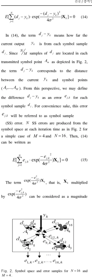
Fig. 2. Symbol space and error samples for N=16 and
=4
M . Fig. 3. Input magnitude controller
0 ] 4 )
) exp( (
) ( [
1 2
2
− =
⋅ −
∑
−= k
N j
k j k
j
y y d
d
E X
σ (14)
In (14), the term dj−yk means how far the current output yk is from each symbol sample dj. Since NM samples of dj are located in each transmitted symbol point Am as depicted in Fig. 2, the term dj−yk corresponds to the distance between the current yk and symbol points (A ,...,1 AM). From this perspective, we may define the difference dj−yk as an error ej,k for each symbol sample d . For convenience sake, this error j
k
ej, will be referred to as symbol sample (SS) error. N SS errors are produced from the symbol space at each iteration time as in Fig. 2 for a simple case of M =4and N=16. Then, (14) can be written as
0 ] 4 )
exp(
[
1 2
2 ,
, − =
∑
⋅= k
N j
k j k
j
e e
E X
σ (15)
The term k
k
ej
X 4 ) exp( 2
2 ,
σ
−
, that is, Xk multiplied
by )
exp(4 2
2 ,
σ
k
ej
−
can be considered as a magnitude
controlled value of Xk according to error values.
For example, when SS error ej,k has a very large value due to some strong noise like impulses, the
exponential )
exp( 4 2
2 ,
σ
k
ej
−
becomes very small (the exponential function is a decay function of SS error power) and the current input Xk is mitigated by the
multiplication of ) exp( 4 2
2 ,
σjk
−e
. This process of input magnitude control is depicted in Fig. 3, defining
MC k
Xj, as a magnitude controlled input.
k k MC j
k j
e X
X )
exp(4 2
2 ,
, σ
= − (16)
With the definition
MC k
Xj, and (12), the MCC algorithm can be rewritten as
∑ ∑
− += =
+ = + k ⋅
N k i
N j
MC i j i j k
k e
N 1, 1
, 3 ,
1 2
2 X
W
W σ π
μ (17)
It is noticed in (17) that the magnitude controlled
MC k
Xj, plays the role in stabilizing the algorithm in situations of large error occurrence when compared with the LMS algorithm in (7) though the two algorithms have a very similar form that comprises error and input.
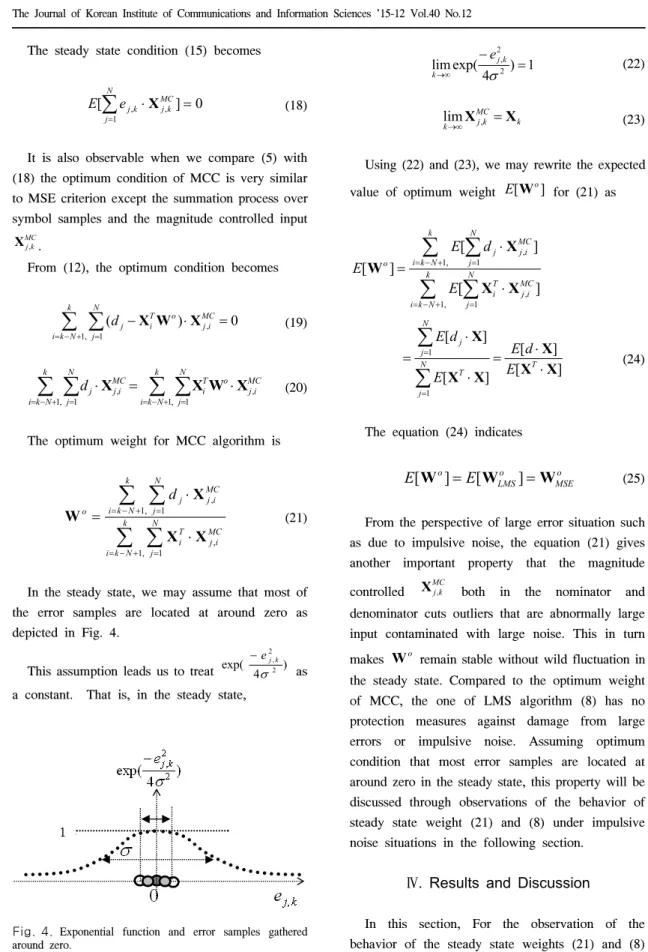
Fig. 4. Exponential function and error samples gathered around zero.
The steady state condition (15) becomes
0 ] [
1
,
, ⋅ =
∑
= N jMC k j k
ej
E X (18)
It is also observable when we compare (5) with (18) the optimum condition of MCC is very similar to MSE criterion except the summation process over symbol samples and the magnitude controlled input
MC k
X . j,
From (12), the optimum condition becomes
0 )
(
,
1 1
, =
⋅
∑ ∑
−+
−
= =
k N k i
N j
MC i j o T i
dj X W X (19)
∑ ∑
∑ ∑
− + =− + == =
⋅
=
⋅ k
N k i
N j
MC i j o T i k
N k i
N j
MC i j
dj
,
1 1
, ,
1 1
, X W X
X (20)
The optimum weight for MCC algorithm is
∑ ∑
∑ ∑
+
−
= =
+
−
= =
⋅
⋅
= k
N k i
N j
MC i j T i k
N k i
N j
MC i j j o
d
,
1 1
, ,
1 1 ,
X X
X
W (21)
In the steady state, we may assume that most of the error samples are located at around zero as depicted in Fig. 4.
This assumption leads us to treat exp( 4 2 )
2 ,
σ
k
ej
−
as a constant. That is, in the steady state,
1 4 ) exp(
lim 2
2
, =
−
→∞ σ
k j k
e (22)
k MC
k
k Xj =X
→∞ ,
lim (23)
Using (22) and (23), we may rewrite the expected value of optimum weight E W[ o] for (21) as
∑ ∑
∑ ∑
+
−
= =
+
−
= =
⋅
⋅
= k
N k i
N j
MC i j T i k
N k i
N j
MC i j j o
E d E E
,
1 1 ,
,
1 1 ,
] [
] [
] [
X X
X
W
] [
] [ ] [
] [
1 1
X X
X X
X X
⋅
= ⋅
⋅
⋅
=
∑
∑
=
=
T N
j T N
j j
E d E E
d E
(24)
The equation (24) indicates
o MSE o
LMS
o E
E[W ]= [W ]=W (25)
From the perspective of large error situation such as due to impulsive noise, the equation (21) gives another important property that the magnitude controlled XMCj,k both in the nominator and denominator cuts outliers that are abnormally large input contaminated with large noise. This in turn makes Wo remain stable without wild fluctuation in the steady state. Compared to the optimum weight of MCC, the one of LMS algorithm (8) has no protection measures against damage from large errors or impulsive noise. Assuming optimum condition that most error samples are located at around zero in the steady state, this property will be discussed through observations of the behavior of steady state weight (21) and (8) under impulsive noise situations in the following section.
Ⅳ. Results and Discussion
In this section, For the observation of the behavior of the steady state weights (21) and (8)
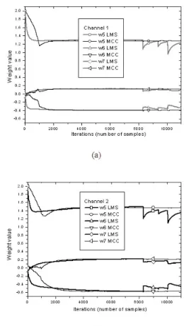
Fig. 6. Trace of weight values in the steady state with impulsive noise for w5,k, w6,k and w7,k(the other weights are not included just for the page-limit); (a) is for channel
)
1(z
H and (b) is for H2(z).
Fig. 5. Background and impulsive noise.
under impulsive noise situations, the channel environment of [7] with the impulse noise being applied in the steady state is used in this paper as depicted in Fig. 5. The symbol point set in the transmitter is
{
d1=−3,d2=−1,d3=1,d4=3}
and a symbol point dk is transmitted at time k through the channel models as
2 1
1(z)=0.26+0.93z− +0.26z−
H (26)
2 1
2(z)=0.304+0.903z− +0.304z−
H (27)
The additive Gaussian white noise (AWGN) is added to the channel output throughout the whole time as a background noise. The impulse noise is added after convergence (8000) as in Fig. 5. The impulsive noise nkis generated according to the following PDF of Gaussian mixture model[3].
2 ] 2 exp[
2 ] 2 exp[
) 1
( 2
2 2
2 2 1 2
1 σ π σ
ε π σ
σ
ε k k
k NOISE
n n n
f = − − + − (28)
where ε , <1 σ1=σGN, σ2= σGN2 +σIN2
The variance σIN2 and incident rate ε of the impulse in this section are given by 50 and 0.01, respectively. The TDL equalizer has 11 weights. The number of random symbol samples N is 32, the
kernel size σ is 0.5.
The convergence step-sizes are μMCC=0.007 for MCC1 and μLMS =0.001 for LMS algorithm. All the parameters are selected to have the lowest steady state MSE in this simulation.
The trace of w5,k, w6,k and w7,k (the other tap weights are not included just for the page-limit) in Fig. 6. The dotted line is the trace of the LMS algorithm and the solid line is the one of MCC1.
Since the steady state weight vectors can be considered to be reached the optimum state, it is reasonable to investigate whether the steady state weights satisfy the relation in (25) and the steady state weight can keep the optimum values under impulsive noise situations. The first thing we can observe in Fig. 6 is that both algorithms have the
same steady state weight values as explained in (25).
Secondly, the weight traces of MCC1, each weight presents no fluctuations staying undisturbed under the strong impulses while the ones of LMS algorithm for all w5,k, w6,k and w7,k show sharp perturbations at each impulse occurrence.
Comparison of (7) and (17) shows that the mainly different terms between the two weight update equations are sample averaging and magnitude controlling processes. Since impulsive noise may defeat the averaging operation as mentioned in Section 2, we can explain that the dominant role in the robustness against impulsive noise is the
magnitude controlled input k
k MC j
k j
e X
X )
exp( 4 2
2 ,
, σ
= −
and therefore the steady state weights of LMS algorithm without the input controlling function cannot avoid wild fluctuations in impulsive noise environment.
Ⅴ. Conclusion
In most blind signal processing applications in impulsive noise environment the MCC algorithm outperforms MSE-based algorithms. However, the optimum solutions and properties related with MCC algorithms have not been sufficiently studied. In this paper, through analysis of the relationship with the behavior of optimum weight of MSE-based LMS algorithm, it has been proven that the optimum weight of MCC is equal to the one of MSE criterion. Furthermore, it is the magnitude controlled input that keeps optimum weight of MCC undisturbed and stable by mitigating the influence of impulsive noise. Studies on application of the magnitude controlled input to enhanced methods are desirable in future research.
References
[1] K. Blackard, T. Rappaport, and C. Bostian,
“Measurements and models of radio frequency impulsive noise for indoor wireless communications,” IEEE J. Sel. Area. Commun., vol. 11, pp. 991-1001, Sept. 1993.
[2] S. Unawong, S. Miyamoto, and N. Morinaga,
“A novel receiver design for DS-CDMA systems under impulsive radio noise environments,” IEICE Trans. Commun., vol.
E82-B, pp. 936 -943, Jun. 1999.
[3] I. Santamaria, P. Pokharel, and J. Principe,
“Generalized correlation function: Definition, properties, and application to blind equalization,” IEEE Trans. Signal Process., vol. 54, pp. 2187-2197, Jun. 2006.
[4] W. Liu, P. P. Pokharel, and J. C. Principe,
“Correntropy: Properties and applications in non-gaussian signal processing,” IEEE Trans.
Signal Process., vol. 55, pp. 5286-5298, Nov.
2007.
[5] N. Kim, S. Kang, and D. Hong, “Blind equalization based on maximum cross- correntropy criterion using a set of randomly generated symbols,” J. KICS, vol. 35, pp. 33- 39, Jan. 2010.
[6] N. Kim, “Practical approach to blind algorithms using random-order symbols and cross-correntropy,” J. KICS, vol. 39A, pp.
149-154, Mar. 2014.
[7] J. Proakis, Digital Communications, McGraw- Hill, 2nd Ed., 1989.
[8] S. Haykin, Adaptive Filter Theory, Prentice Hall, Upper Saddle River, 4th Ed., 2001.
[9] E. Parzen, “On the estimation of a probability density function and the mode,” Ann. Math.
Stat., vol. 33, p. 1065, 1962.
김 남 용 (Namyong Kim)
1986년 2월:연세대학교 전자 공학과 졸업
1988년 2월:연세대학교 전자 공학과 석사
1991년 8월 : 연세대학교 전자 공학과 박사
1992년 8월~1998년 2월:관동대 학교 전자통신공학과 부교수 1998년 3월~현재 : 강원대학교 공학대학 전자정보통
신공학부 교수
<관심분야> Adaptive equalization.