Evaluating the Soil Salinity of Reclaimed Wastewater Irrigation in Paddy Plots using the Soil-Water-Atmosphere-Plant Model and Water Management Response Indicators
하수처리수의 재이용에 따른 SWAP 모형과 물관리반응지수를 이용한 논에서의 토양염분 평가
Jang, Taeil*
․Hwang, Syewoon
**,†․Jeong, Han Seok
***․Kang, Moon Seong
****․Park, Seung Woo
****장태일․황세운․정한석․강문성․박승우
ABSTRACT
본 연구에서는 하수재이용에 따른 논에서의 토양염분 변화를 추정하기 위하여 경기도 화성시 수원환경사업소 인근에 위치한 병점지구 를 대상으로 수문순환과 작물성장과의 관계를 고려한 SWAP (Soil-Water-Atmosphere-Plant) 모형을 이용하여 평가하였다. 실험에 사용한 관개용수는 지하수 (TR#1), 하수처리장 방류수+여과+UV (TR#3)로 분류하여 모형에 사용하였다. 유입관개수의 EC (Electrical Conductivity) 는 지하수 관개수인 TR#1이 다른 처리구에 비해 작았고, TR#3의 경우 0.442~0.698 dS m-1의 범위를 보였다. 모형의 보정과 검정을 위 해서 대상지구에 FDR (Frequency Domain Reflection)을 설치하여 토양수분함유량과 염분농도를 토심에 따라 일단위로 모니터링 하였다.
토심 (50, 100, 140 cm)에 따른 토양함수량의 RMSE는 검정기간 중 TR#1에서 0.003~0.064 cm3 cm-3, TR#3에서 0.001 cm3 cm-3 범위를 보여 주었고, 토양염분의 보정기간 중 토심별 RMSE는 TR#1에서 0.018~0.037 dS m-1, TR#3에서 0.004~0.014 dS m-1 범위 를 보여 적용성이 있는 것으로 나타났다. 토양내의 염분수지 분석 결과, 토양에서의 염분저장량이 (−)로 나타나 토양내로 침출되는 것으 로 나타났으며, WMRI (Water Management Response Indicators)을 이용한 분석 결과, 높은 침투능으로 인하여 토양에서의 염분 집적 영 향은 낮은 것으로 평가되었다.
Keywords: Reuse; Soil salinity; Soil moisture content; SWAP; Salt storage index
I. INTRODUCTION*
Rice is the most wide-cultivated crops and staple food for about 3 billion people in the world (Govindarajan et al., 2008). South and South-East Asia may suffer economic water scarcity for approximately 22 million ha of irrigated dry-season paddy fields by 2025 (Tuong and Bouman, 2003).
Most countries have suffered from a limited water supply, including agricultural irrigation water, due to population
* Department of Biological & Agricultural Engineering, University of Georgia, USA/Research Institute for Agricultural & Life Sciences, Seoul National University
** Water Institute, University of Florida, USA
*** Rural Systems Engineering, College of Agricultural & Life Science, Seoul National University
**** Rural Systems Engineering, Research Institute for Agricultural &
Life Sciences, College of Agricultural & Life Science, Seoul National University
† Corresponding author Tel.: +1-352-392-5893 Fax: +1-352-392-6855
E-mail: [email protected] 2012년 1월 27일 투고 2012년 3월 8일 심사완료 2012년 3월 13일 게재확정
growth, urbanization, and economic development (IWMI, 2002).
A recent national survey on the future Korean water supply and demand reported that the country can expect a shortage of over 0.44 billion m3 of water by 2030 (MLTM, 2006).
Paddy rice production requires large amounts of water.
For instance, agricultural irrigation is allocated upwards of 47 % of the total annual water use in Korea (Jang et al., 2012). Reclaimed wastewater can be an alternative water resource for supplementary irrigation in areas that suffer from water shortages or unsatisfactory water quality since agricultural irrigation water is not usually required to meet same high standards of water quality as drinking water (Kang et al., 2007; Jang et al., 2010; 2012). From this reason, guidelines for reclaimed wastewater irrigation have been developed by Ministry of Agriculture and Forestry (MAF) and Ministry of Environment (MOE) with the super- vision of Seoul National University, and MOE finally adopted one for paddy fields irrigation in Korea (MOE, 2005). As a result, more data (i.e., water quality and soil) are getting available and help clarify potential human health problems
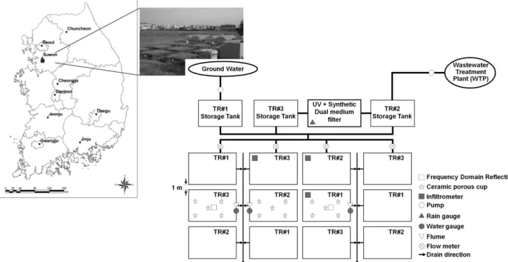
Fig. 1 Location and schematic representation of the study site and field experiments including the wastewater reclamation and irrigation system and water sampling gauges (Jang et al., 2012)
and assess the environmental effects associated with re- claimed wastewater irrigation of paddy fields. However, few reports of practical wastewater reuse for rice paddies have been presented (Kang et al., 2007; Jang, 2009; Jang et al., 2008; 2010; 2012) while case studies for upland crop irrigated with treated wastewater have been reported in many countries (Jang et al., 2012).
A high concentration of sodium in wastewater might cause damage the physico-chemical properties of paddy soil and the close investigation of the soil environment is needed.
Bond (1998) pointed out that the effects of increasing soil salinity and sodicity on current and future land are one of the key limitations on sustainable wastewater irrigation.
Aljaloud et al. (1993) showed that irrigating with wastewater increased maize crop yield when a water salinity level is less than 2330 mg L-1. Numerous studies (Robbins and Lehrsch, 1992; Abu-Sharar, 1996; Stevens et al., 2003;
Angin et al., 2005; Lehrsch et al., 2008; Muyen et al., 2011) have shown that treated or untreated wastewater has the potential to improve the structural properties of soils and increase agricultural productivity. Additionally the systematic monitoring would be also important in order to identify
the cumulative effects of long-term wastewater irrigation on soil chemical and physical properties (Buckland et al., 2002). Few researches for reclaimed wastewater irrigation in paddy fields, however, have reported the effects on soil salinity (Jang, 2009; Jang et al., 2010).
The objectives of this study are to investigate the chemical characteristics on water and soil in paddy plots irrigated by groundwater, wastewater, and reclaimed wastewater and assess the soil salinity of reclaimed wastewater irrigation in paddy plots using the agro-hydrological model and water management response indicators.
II. Material and methods
1. Experimental Site and Design
The experimental paddy plots (E 37˚ 12’ 32’’, N 127˚
01’ 18’’) are located near the Suwon wastewater treatment plant in Gyeonggi-do, Korea. A randomized complete block designed with split plot arrangements was used for three treatments and four replicates with 5 m × 5 m plots (Fig. 1).
The three treatments indicate the different irrigation water used for plots: groundwater (TR#1), untreated wastewater
(TR#2), and filtered wastewater with ultraviolet (UV) treat- ment (TR#3). A small scale wastewater reclamation system with a LCHE-WRT filter system (Maeng et al., 2006), UV treatment unit, and pipelines supply irrigation water from the wastewater effluents. A groundwater well was installed to supply water for TR#1.
For this experiment, 1-month-old rice seedlings (
Oryza sativa cv. Chucheongbyeo
) were transplanted into the study plots in May and harvested in October during the study period. Fertilizers are typically applied three times, during the pre-plant, tilling, and panicle growing stages, but for our experiment, applied one time during the pre-plant (N:P:K=55:45:40 kg ha-1) based on high-nutrient- concentration irrigation. Insecticides were sprayed in June of every year to exterminate rice water weevils, and weeds were controlled manually. This study was conducted for three crop-years from 25 May, 2006 to 21 October, 2008.
2. Soil-Water-Atmospheric-Plant (SWAP) Model
SWAP (soil-water-atmosphere-plant) is an agro- hydrological model developed by Feddes et al. (1978), van Dam et al. (1997), and Kroes and van Dam (2003).
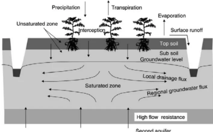
Hydrological processes of the model are shown in Fig. 2.
SWAP calculates water and salt balances of cropped soil columns. In this study the model was used to evaluate the effects of water and salt in the soil columns. Using deterministic and physical laws, SWAP simulates variably saturated water flow, solute transport, and heat flow in unsaturated/saturated soils in relation to crop development
Fig. 2 Hydrological process in Soil-Water-Atmosphere-Plant (SWAP) model (van Dam et al., 2008)
(van Dam et al., 2008). SWAP provides a wide variety of experimental simulations to address practical questions in agricultural water management and environmental protection (Govindarajan et al., 2008; van Dam et al., 2008). The version used for this study is SWAP 3.2 and brief de- scription of the model is presented following. More detailed on the model structure and physics have been well-described by van Dam et al. (1997, 2008).
Transport processes are considered at the field-scale level according to whole growing season. Upper boundary in the model is defined as the atmospheric conditions at soil surface with/without crop conditions. The upper boundary condition also includes runoff calculations and allow to alternate conditions of a shallow groundwater table and surface ponding depth. Bottom boundary is located in unsaturated zone or upper part of groundwater table. SWAP uses Richards’ equation with sink and source terms to simulate water movement in both the unsaturated and saturated zone:
(1)
where, is volumetric water content (-), is time (T), is hydraulic conductivity (L T-1), h is soil water pressure head (L), is vertical coordinate (L, positive upward), and S is a source-sink term (T-1) that accounts for root water extraction, lateral drainage, and/or water exchange in soil matrix.
SWAP model is linked with crop growth module, which is based on the world food studies (WOFOST) model (Spitters et al. 1989; Supit et al. 1994). This model simulates the crop growth and its production based on the incoming photosynthetically active radiation absorbed by the crop canopy and the photosynthetic characteristics of leaf. Addi- tionally the model accounts for water and salt stress of the crop (Govindarajan et al., 2008).
3. Data Collection
In this study, climate data, soil data, irrigation records, and plant growth details were collected from 2006 to 2008
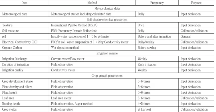
Table 1 Overview of the data collected for calibrating and validating the SWAP model
Data Method Frequency Purpose
Meteorological data
Meteorological data Meteorological station including calculated data Daily Input derivation Soil physio-chemical properties
Texture International Pipette Method (USDA) Once Input derivation
Soil moisture FDR (Frequency Domain Reflection) Daily Calibration/validation
pH In soil-water suspension of 1:5 by pH meter Before and after irrigation General
Electrical Conductivity (EC) FDR/In soil-water suspension of 1:2 by Conductivity meter Daily/weekly Calibration/validation
Organic Carbon Wet digestion method Before sowing Input derivation
Irrigation regime
Irrigation Discharge Current meter/Flow meter Weekly Input derivation
Duration of irrigation Field observation Each irrigation Input derivation
Irrigation quality Conductivity meter Weekly Input derivation
Crop growth parameters
Crop development stage Field observation 5-6 times Input derivation
Plant density and tillers Field observation 5-6 times Input derivation
Plant height Field observation 5-6 times Input derivation
Leaf area Leaf area meter 5-6 times Calibration/validation
Rooting depth Field observation, Auger method 4-5 times Input derivation
Crop yields Field observation at Harvest Calibration/validation
to run the SWAP model. Table 1 shows the overview of data collected for running the SWAP model in this experi- mental plot. The calibration process for hydraulic parameters was performed with the first part of observations (June-July) and the second part of observations (Aug.-Sep.) was used for the validation.
a. Meteorological data
The required climate data to run the simulation was collected from the nearest weather station to the study area, the Suwon National Meteorological Station. It includes daily rainfall, average daily maximum and minimum tem- perature, daily relative humidity, and daily wind velocity.
Daily radiation was calculated using the Hargreaves radiation formula given by Allen et al. (1998). The annual mean temperature and total rainfall during the irrigation periods showed 22.1 °C and 1032.4 mm for 2006, 21.4 °C and 995.0 mm for 2007, 22.0 °C and 1098.8 mm for 2008, respectively.
b. Soil data
In order to solve the Richard’s equation, the soil physical characteristics, soil retention and hydraulic conductivity curves should be known. Soil samples were collected from
Table 2 Physical and chemical properties of the soil in the experimental plots (Jeong et al., 2011)
Properties Unit TR#1 TR#2 TR#3
Sand
%
48.7 48.7 48.7
Silt 32.3 35.3 30.8
Clay 19.0 16.0 20.5
Texture class - Loam Loam Loam
Organic matter % 1.74 2.11 1.82
pH (1:5) - 5.55 5.52 5.53
CEC cmol+ kg-1 13.09 12.11 13.29
EC μS/m 0.473 0.319 0.524
TN
mg kg-1
850.0 930.0 950.0
TP 528.2 557.7 358.3
Ca 758.5 853.8 745.2
K 40.9 44.5 49.5
experimental plots before transplanting and after harvesting.
After clearing organic matter from the surface, three soil sub-samples were taken from the root zone (2−30 cm below the soil surface) and 60 cm depth of soil at each plot. The soil samples were analyzed for physical and chemical properties with the American Society of Agronomy (ASA) and Soil Science Society of America (SSSA) methods for soil analysis (Chapman and Pratt, 1961). Bulk density
was measured by sand replacement method and percentage organic carbon was estimated. The measured soil charac- teristics obtained from field experiment and data reported by the literature by Jang (2009) and Jeong et al. (2011) are given in Table 2.
c. Crop growth data
The growing stages for rice were recorded by measuring the crop height, leaf area index (LAI) and dry matter. The plant height was measured from the soil surface to the top of the straightened shoot/leaf. Leaf area was measured for two plant hills in each plot. At the time of harvesting, crop cutting experiment was conducted. After manual threshing, the grain and straw weights were monitored.
d. Irrigation data
The amounts of water irrigated to the plots were me- asured using an automatic float type water level recorder.
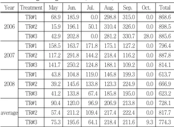
Inflow and outflow were measured using a water gauge at the inlet pipe and outflow was measured using weirs in- stalled at the outlet of three plots, respectively. These data were used as input for the model to specify the bottom boundary conditions. Table 3 presents the monthly irrigation amounts and Table 4 shows the Electrical Conductivity (EC) characteristics of rainfall and irrigation water for each experimental plot during study period from 2006 to 2008.
The differences of irrigation amounts according to the treatments may have been affected by different hydrologic
Table 3 Monthly irrigation amount in the experimental plots for growing season (unit: mm)
Year Treatment May Jun. Jul. Aug. Sep. Oct. Total
2006
TR#1 68.9 185.9 0.0 298.8 315.0 0.0 868.6 TR#2 15.9 196.1 50.1 310.4 326.0 0.0 898.5 TR#3 42.9 202.8 0.0 281.2 330.7 28.0 885.6
2007
TR#1 158.5 163.7 171.8 175.1 127.2 0.0 796.4 TR#2 117.2 291.8 144.2 218.4 116.2 0.0 887.8 TR#3 141.7 250.2 124.8 188.1 109.2 0.0 814.1
2008
TR#1 43.8 104.8 119.0 146.8 199.3 0.0 613.7 TR#2 39.2 145.6 133.8 123.3 224.9 0.0 666.9 TR#3 41.2 133.8 67.4 185.8 195.0 0.0 623.2
average
TR#1 90.4 120.0 96.9 206.9 213.8 0.0 728.1 TR#2 57.4 211.2 109.4 217.4 222.4 0.0 817.7 TR#3 75.3 195.6 64.1 218.4 211.6 9.3 774.3
Table 4 Electrical Conductivity (EC) concentration charac- teristics of rainfall and irrigation water for the study period
Samples Rainfall water (dS m-1)
Irrigation water (dS m-1)
TR#1 TR#2 TR#3
Mean 0.249 0.378 0.532 0.545
Max 0.584 0.772 0.915 0.830
Min 0.079 0.176 0.070 0.338
Standard Deviation 0.182 0.073 0.140 0.112
Number 11 53 53 53
The rainfall sampling period was during 2008.
and soil conditions and different irrigation intensities of the three irrigation systems (Jang et al., 2012). The soil moisture and salinity were monitored on daily-basis at the 50, 100, and 140 cm of soil depth using FDR (Frequency Domain Reflection) (Hong et al., 2011).
4. Model Estimation
Water flow and salt transport are very sensitive to the soil hydraulic functions of () and () (Singh et al., 2006; Govindarajan et al., 2008). We performed automatic calibration, which is also known as inverse modeling. A non-linear parameter estimation program PEST (Doherty et al., 2004) was linked with SWAP model. The soil moisture and salinity profiles observed at different depth were used to calibrate the soil hydraulic parameters. The measured crop growth was also used in the calibration process.
As quantitative criteria for evaluating the model perfor- mance, the root mean square error (RMSE) was used to examine the feasibility of the model. The RMSE is an ab- solute error measure quantifying the error in terms of the unit of variable. The objective function quantifies the di- fferences between model results and observations as follows:
(2)
where, () and () are the observed and simulated soil moisture and salinity at time , respectively. is the number of observations.
Table 6 Calibrated soil hydraulic parameters between two treatments at each soil depth
Soil layer (cm) Texture
Soil hydraulic parameters
r es (cm3 cm-3)
sat (cm3 cm-3)
sat (cm d-1)
(cm-1)
(−)
(−)
TR#1 TR#3 TR#1 TR#3 TR#1 TR#3 TR#1 TR#3 TR#1 TR#3 TR#1 TR#3
10-50 L 0.078 0.078 0.14 0.17 5.34 5.34 0.021 0.005 -2.97 -2.97 2.580 1.098
50-100 L 0.078 0.078 0.45 0.41 5.24 5.24 0.004 0.019 -2.37 -2.37 2.483 1.470
100-140 SL 0.067 0.067 0.30 0.28 4.45 4.45 0.015 0.005 -1.55 -1.55 1.499 1.480
5. Water management response indicators
The crop yields may indicate the success or failure of irrigation and drainage, but they provide no information on the environmental sustainability (Molden and Gates, 1990;
van Dam and Malik, 2003). In order to quantify this issue, we used the Water Management Response Indicators (WMRI), which is suggested by Bastiaanssen et al. (1996). WMRI indicates the intensity of water and salt stress on the crop.
It consists of irrigation contribution index, percolation index, and salt storage index. The percolation index indicates the leaching fraction and therefore the salinization or water- logging risk. The salt storage index expresses the salt build up in the root zone. For a sustainable system, the salt storage change must be near zero or negative over a long period (van Dam and Malik, 2003).
Irrigation contricbution index (ICI)=IR/ETa (3) Percolation index (PI)=Qbot/IR (4)
Salt stroage index=ΔC/C (5)
where, IR is irrigation water amounts (mm), ETa is the actual evapotranspiration (mm), Qbot is deep percolation (mm,+upward), and C and ΔC (g cm-3) are the initial value and change of salt storage in the soil profile, respectively.
III. RESULTS AND DISCUSSION
1. Parameter Estimation
In this study, we focused on two treatments, TR#1 and TR#3, because the irrigation of wastewater effluent (i.e., TR#2) is not applied for actual irrigation. The nutrient
concentrations for TR#2 are slightly higher than for TR#3 and there is no significant difference between the EC concentrations for TR#2 and TR#3. In addition, we are not currently addressing a primary objective for evaluating irrigation with wastewater effluent.
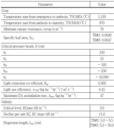
The input parameters of SWAP could be categorized by the upper boundary, crop, soil, and initial conditions. The input parameters used in this study are summarized in Table 5.
The soil moisture and salinity profiles observed during the growing season were used for the calibration and validation of soil hydraulic parameters. Soil hydraulic para- meters and for the different soil layers of stratified
Table 5 Main crop parameters specified for SWAP model for rice
Parameter Value
Crop
Temperature sum from emergence to anthesis, TSUMEA (℃) 1,150 Temperature sum from anthesis to maturity, TSUMAM (℃) 970 Minimum canopy resistance, rcrop (s m-1) 70
Specific leaf area, SLA TR#1: 0.0020
TR#3: 0.0047 Critical pressure heads, h (cm)
h1 100
h2 55
h3l -160
h3h -250
h4 -16,000
Light extinction co-efficient, Kgr 0.300
Light use efficiency, PAR (kg ha-1 hr-1/ J m2 s-1) 0.45 Maximum CO2 assimilation rate, Amax (kg ha-1 hr-1) 47 Salinity
Critical level, ECmax (dS m-1) 3.0
Decline per unit EC, EC slope (dS m)-1 11.0
Dispersion length, Ldis (cm) TR#1: 5.0~5.5
TR#3: 5.5~50.0
soil profile were calibrated simultaneously. Repetition of the optimization process with different initial values of and resulted in the same values, which showed the uniqueness of the solution. The calibrated values of and
together with the other soil hydraulic parameters (res,
sat, sat, and ) are given in Table 6.
2. Model Evaluation
The procedure of SWAP model evaluation followed the sequence of soil moisture () and soil EC, LAI, and crop yield in this study. However, the period of validation applied with two approaches: (1) the calibration and verification of , EC, and LAI was conducted in 2008 due to the limitation of monitoring data and model input, and (2) that of crop yield was performed from 2006 to 2008 in each treatment.
Table 7 presents the RMSE values of and EC values in the soil profile for the study period. The average RMSE of for calibrated and validated period ranged from 0.001 to 0.064 cm3 cm-3 for TR#1 and from 0.001 to 0.006 cm3 cm-3 for TR#3, respectively. The average RMSE of at the 140 cm depth of soil in the TR#3 showed relatively high with 0.064 cm3 cm-3. Overall, the simulation results in this study showed reasonable agreement with the observed data.
The average RMSE of EC for calibrated and validated period ranged from 0.001 to 0.037 dS m-1 for TR#1 and ranged from 0.004 to 0.045 dS m-1 for TR#3, respectively.
The average RMSEs of EC were larger than those of . This result has reasonable agreement comparing to the
Table 7 Observation numbers and root mean square (RMSE) of soil moisture contents () and soil salinity (EC) in the experimental plots
Treatment Soil layer (cm)
Calibrated Validated
No.
(cm3 cm-3)
EC (10-3 dS m-1) No.
(cm3 cm-3)
EC (10-3 dS m-1)
RMSE RMSE RMSE RMSE
TR#1 50
57
0.002 0.023
57
0.003 0.037
100 0.002 0.023 0.003 0.037
140 0.001 0.001 0.064 0.018
TR#3 50
45
0.002 0.033
46
0.001 0.004
100 0.002 0.045 0.001 0.014
140 0.006 0.028 0.001 0.004
measurement data presented by Singh et al. (2006). This might be caused by the persistent ponding-status by the irrigation and/or rainfall during the growing season.
The measured leaf LAI for two treatment plots are given in Fig. 3. In the TR#1, the maximum LAI was estimated by 3.65 in mid-August and 9.45 for the TR#3 at same season.
The LAI for the TR#3 was greatly estimated to be higher than that for the TR#1 likely because of the high-nutrient- concentration irrigation. The coefficients of determination (R2) for LAI of two treatments were 0.94 for TR#1 and 0.98 for TR#3, respectively.
The crop yields are shown in Fig. 4 and the same trend as in the LAI development was observed. The average yield for TR#3 was about 15 % greater than for TR#1 and this was greater than the national average yield (4,500 kg
․ ha-1) in Korea as well (Jung, 2011; Jang et al., 2010;
Fig. 3 Observed and simulated leaf area index (LAI) between two treatments
Fig. 4 Observed and simulated crop yield between two treatments for the study period
2012). This implies there is the fertilization reduction effect when reclaimed wastewater is used for irrigation compared to conventional irrigation and fertilization. The yield of TR#1, however, was underestimated in 2008 and that of the TR#3 was overestimated. Overall, the R2 for average rice yield in two treatments was 0.88 and it showed re- asonable agreement with the observed data.
3. Water and Salt Balances
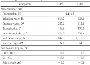
The calibrated soil hydraulic parameters (see, Table 6) along with other inputs were used to simulate the water and salt balances in two paddy plots. The water and salt balances simulated by the SWAP are presented in Table 8. The averaged simulated results show irrigation of 614 to 623 mm, rainfall of 1111 mm, ET of 459 to 479 mm, and infiltration of 1,018 to 1,048 mm, and about 13 % of infiltration was drained by surface drainage. The average drainage amount was far lower in this study than in other studies (Jang et al., 2012), due to the high drainage outlet height; we used the flume of the outlet, which was designed with a V-notch positioned above 15 cm from the base in order to maintain a constant outlet height. The water balance analysis indicates that approximately 30 % was consumed by crop harvest and 40 % was lost by evapotranspiration and infiltration. The soil salt storage, ΔC, was negative
Table 8 Computed water and salt balances during the agricultural activity
Component TR#1 TR#3
Water balance (mm)
Precipitation, PR 1,110.5
Irrigation water, IR 613.7 623.2
Drainage water, DR 235.2 311.3
Transpiration, T 138.9 136.4
Evapotranspiration, ET 478.6 459.2
Infiltration water, IN 1,047.5 1,018.0
water storage, ΔW 37.1 54.8
Salt balance (mg cm-2)*
(IR+PR) ․ Ci 14.4 17.5
Qbot․ Cbot -16.1 -17.6
Salt storage, ΔC -1.7 -0.1
* Qbot and Cbot are water percolation at the soil column bottom and salt bottom flux, respectively.
Height soil column is assumed with 250 cm.
Table 9 Annual computed water management response in- dicators (WMRI)
Treatment WMRI
ICI PI SI
TR#1 1.50 -2.67 -6.03
TR#3 1.75 -3.28 -0.29
Other studies (van Dam et al., 2003) 1.21 -0.28 0.44
1.07 -0.20 -0.10
indicating that the soil salt storage decreased by leaching during growing season in both treatment plots, that is, the soil salt is not accumulated in the soil profile.
Table 9 shows the indices (equation 3-5) of WMRI for each experimental plot. The annual percolation index for two treatments was relatively high compared to the previous studies (Singh et al., 2006). It likely resulted from soil characteristics of the plots (i.e., sandy-loam having good drainage capacity). The percolation index indicates water is not accumulated and leached in the soil profile, which is also clear from the salt storage index. The average EC concentration of two treatments was 0.38 dS m-1 for TR#1 and 0.50 dS m-1 for TR#3, respectively. These EC levels indicate that there is no salt stress for the rice growth during the experiment periods (Jang, 2009). In addition, negative salt storage index in both treatments (-0.29 and
-6.03) implies that the salinity concerns is not adversely affected by leaching of salt, however, long-term monitoring may be needed to observe and understand for the potential concerns of secondary salinization in the future.
IV. CONCLUSIONS
Reclaimed wastewater reuse in agriculture has been considered to be an alternative agricultural water resource because of its potential economic and environmental bene- fits, although it is still under challenging to increase the benefit of reclaimed wastewater reuse and decrease the environmental and health risks. This research found that reclaimed wastewater could be used for rice paddy irrigation with no adverse impacts on the paddy soil environment. In order to derive water and salt balances of reclaimed waste- water reuse, the SWAP model was used and the calibration and validation results showed the good agreement between
simulated and observed in soil moisture and EC for the calibrated and validated period. The percolation and salt storage indexes were estimated to be negative indicating salt buildup in the soil profile could be leached. In addition, reclaimed wastewater showed relatively low sodium con- centration where the rice growth and soil environment are not affected. This study would be limited by spatiotemporal constraints (e.g., filed scale experiment and 3-year period) and this, longer-term study would be required to obtain general conclusion. Furthermore, there is necessarily to study various wastewater effluent and soil characteristics reflecting the local features in order to safe and sound reuse of agricultural culture.
This project was supported by the Technology De- velopment Program for Agriculture and Forestry, Ministry for Food, Agriculture, Forestry and Fisheries, Republic of Korea. Funding of this research was also provided by a grant (code# 4-5-3) from the Sustainable Water Resources Research Center of the 21st Century Frontier Research Program.
REFERENCES
1. Abu-Sharar, T. M., 1996. Modification of hydraulic properties of a semiarid soil in relation to seasonal applications of sewage sludge and electrolyte-producing compounds.
Soil Technology
9: 1-13.2. Aljaloud, A. A., G. Hussain, A. J. Alsaati, and S.
Karimullah, 1993. Effects of wastewaters on plant growth and soil properties.
Arid Soil Research and Rehabilitation
7: 173-179.3. Allen, R. G., L. S. Pereira, D. Raes, and M. Smith, 1998. Crop evapotranspiration. Guidelines for computing crop water requirements.
FAO Irrigation and Drainage Paper
No. 56, Rome, Italy.4. Angin, I., A. V. Yaganoglu, and M. Turan, 2005. Effects of long-term wastewater irrigation on soil properties.
Journal of Sustainable Agriculture
26: 31.5. Bastiaanssen, W. G. M., R. Singh, S. Kumar, J. K.
Schakel, and R. K. Jhorar, 1996. Analysis and re- commendations for integrated on-farm water management
in Haryana, India: a model approach. Report 118, DLO Winand Staring Center, Wageningen. 152 pp.
6. Bond, W. J., 1998. Effluent irrigation - an environmental challenge for soil science.
Australian Journal of Soil Research
36: 543-555.7. Buckland, G. D., D. R. Bennett, D. E. Mikalson, Ed. Jong, and C. Chang, 2002. Soil salinization and sodification from alternate irrigations with saline-sodic water and simulated rain.
Canadian Journal of Soil Science
82:297-309.
8. Chapman, H. D. and P. F. Pratt, 1961.
Methods of analysis for soils, plants and waters.
University of California: Division of Agricultural Sciences, CA.9. Doherty, J., L. Brebber and P. Whyte, 2004.
PEST:
Model independent parameter estimation: user manual 5th edtion.
Australian Centre for Tropical Freshwater Research, James Cooke University, Townsville, Australia.10. Feddes, R. A., P. J. Kowalik, and H. Zaradny, 1978.
Simulation of field water use and crop yield. Simulation Monographs, Pudoc, Wageningen, The Netherlands, 189 p.
11. Govindarajan, S., N. K. Ambujam, and K. Karunakaran, 2008. Estimation of paddy water productivity (WP) using hydrological model: an experimental study.
Paddy and Water Environment
6: 327-339.12. Hong, E. M., J. Y. Choi, W. H. Nam, and S. H. Yoo, 2011. Analysis of soil moisture recession characteristics in Conifer forest.
Journal of the Korean Society of Agricultural Engineering
53:1-9 (in Korean).13. IWMI, 2002. Urban Wastewater: A Valuable Resource for Agriculture: A Case Study from Haroonabad, Pakistan: Research Report 63: International Water Management Institute (IWMI): Colombo, Sri Lanka. 21.
14. Jang, T. I., 2009. Environmental effects of reclaimed wastewater irrigation on paddy fields. Doctoral Dis- sertation, Seoul National University, Seoul, Korea (in Korean).
15. Jang, T. I., H. K. Kim, C. H. Sung, E. J. Lee, and S.
W. Park, 2012. Assessing nutrient losses of reclaimed wastewater irrigation in paddy fields for sustainable agriculture.
Agricultural Water Management
104: 235- 243.16. Jang, T. I., S. B. Lee, C. H. Sung, H. P. Lee, and S. W.
Park, 2010. Safe application of reclaimed water reuse for agriculture in Korea. Paddy and Water Environment 8: 227-233.
17. Jang, T. I., S. W. Park, and H. K. Kim, 2008.
Environmental effects analysis of a wastewater reuse system for agriculture in Korea.
Water Science and Technology: WS
8: 37-42.18. Jeong, H. S., C. H. Seong, T. I. Jang, K. W. Jung, M.
S. Kang, and S. W. Park, 2011. Effects of reclaimed wastewater irrigation on paddy rice yields and fertilizer reduction using the DSSAT Model.
Journal of the Korean Society of Agricultural Engineers
53: 67-74 (in Korean).19. Jung, K. W., 2011. Effects of reclaimed wastewater irrigation on paddy rice growth and yield. Mater thesis, Seoul National University, Seoul, Korea (in Korean).
20. Kang, M. S., S. M. Kim, S. W. Park, J. J. Lee, and K.
H. Yoo, 2007. Assessment of reclaimed wastewater irrigation impacts on water quality, soil, and rice cultivation in paddy fields.
Journal of Environmental Science and Health Part A
42: 439-445.21. Kroes, J. G. and J. C. van Dam (eds), 2003. Reference Manual SWAP version 3.03. Alterra Green World Research, Alterra report 773, ISSN 1566-7197.
Wageningen University and Research Centre, Wageningen, Netherlands.
22. Lehrsch, G. A., C. W. Robbins, and M. J. Brown, 2008. Whey utilization in furrow irrigation: effects on aggregate stability and erosion.
Bioresource Technology
99: 8458-8463.23. Maeng, S. K., K. H. Ahn, K. P. Kim, K. G. Song, and K. Y. Park, 2006. Compressible synthetic dual-medium filtration of wastewater effluents for water reuse.
Water Practice and Technology
1: doi10.2166/wpt.2006.050.24. MLTM, 2006. Water Vision 2020 (2006 National Water Resources Plan Update). Ministry of Land, Transportation and Maritime Affaris (MLTM). Kyeonggi-do, Korea.
Available at: www.waterplan.go.kr. Accessed 25 August 2011 (in Korean).
25. MOE, 2005. Recommended Water Quality Guidelines for Wastewater Reuse. Ministry of Environment (MOE).
Gyeonggi-do, Korea (in Korean).
26. Molden, D. J. and T. K. Gates, 1990. Performance
measures for evaluation irrigation water-delivery systems.
Journal of Irrigation and Drainage Engineering
116: 804-823.27. Muyen, Z., G. A. Moore, and R. J. Wrigley, 2011. Soil salinity and sodicity effects of wastewater irrigation in South East Australia.
Agricultural Water Management
99: 33-41.28. Robbins, C. W., and G. A. Lehrsch, 1992. Effects of acidic cottage cheese whey on chemical and physical properties of a sodic soil.
Arid Soil Research and Rehabilitation
6: 127-134.29. Singh, R., J. C. van Dam, and R. A. Feddes. 2006.
Water productivity analysis of irrigated crops in Sirsa district, India.
Agricultural Water Management
82: 253- 278.30. Spitters, C. J. T., H. van Keulen, and D. W. G. van Kraalingen, 1989.
A simple and universal crop growth simulator: SUCROS87.
In: R. Rabbinge, S. A. Ward and H. H. van Laar (Eds.). Simulation and systems management in crop protection. Simulation Monographs.Wageningen, Pudoc, The Netherlands, 147-181.
31. Stevens, D. P., M. J. McLaughlin, and M. K. Smart, 2003. Effects of long-term irrigation with reclaimed water on soils of the Northern Adelaide Plains, South Australia.
Australian Journal of Soil Research
41: 933- 948.32. Supit, I., A. A. Hooijer, and C.A. van Diepen (Eds.), 1994. System description of the WOFOST 6.0 Crop Growth Simulation Model implemented in CGMS. Volume 1: Theory and algorithms. European commission, Luxembourg. 146 pp.
33. Tuong, T. P. and B. A. M. Bouman, 2003.
Rice production in water-scarce environments. In J. Kijne, R. Barker and D. Molden (Eds.),
Water productivity in agriculture: limits and opportunities for improvement, CABI press, Wallingford, UK.34. van Dam J. C., and R. S. Malik, 2003. Water productivity of irrigated crops in Sirsa district, India. Integration of remote sensing, crop and soil models and geographical information systems. WATPRO final report, including CD-ROM. ISBN 90-6464-864-6.
35. van Dam, J. C., 2000. Field-scale water flow and solute
transport. SWAP model concepts, parameter estimation and case studies. Wageningen University, Netherlands.
36. van Dam, J.C., P. Groenendijk, R. F. A. Hendriks, and J. P. Kroes, 2008. Advances of Modeling Water Flow in Variably Saturated Soils with SWAP.
Vadose Zone Journal
7: 640-653.37. van Dam, J. C., J. Huygen, J. G. Wesseling, R. A.
Feddes, P. Kabat, P. E. V. van Walsum, P. Groenendijk, and C. A. van Diepen. 1997. Theory of SWAP version 2.0. Simulation of water flow, solute transport and plant growth in the Soil. Water. Air. Plant environment.
Technical Doc. 45. Alterra, Wageningen, the Netherlands.