2003, Vol. 14, No.4 pp. 1091∼1102
A Note on Estimating Parameters in The Two-Parameter Weibull Distribution
Mezbahur Rahman1) ․ Larry M. Pearson2)
Abstract
The Weibull variate is commonly used as a lifetime distribution in reliability applications. Estimation of parameters is revisited in the two-parameterWeibull distribution. The method of product spacings, the method of quantile estimates and the method of least squares are applied to this distribution. A comparative study between a simple minded estimate, the maximum likelihood estimate, the product spacings estimate, the quantile estimate, the least squares estimate, and the adjusted least squares estimate is presented.
Key Words : Least squares estimate; Maximum likelihood estimate;
Method of product spacings estimate; Quantile estimate; Simple minded estimate.
Running Title : Weibull Parameter Estimation
1. Introduction
The random variable X has a Weibull distribution with two parameters and η if it has a probability density function of the form:
f (x ) = η
x
η
− 1
e−
x
η ; > 0, η > 0 (1)
1) Department of Mathematics and Statistics, Minnesota State University, Mankato, MN 56002, USA
E-mail : [email protected]
2) Department of Mathematics and Statistics, Minnesota State University, Mankato, MN 56002, USA
E-mail : [email protected]
The distribution function of the Weibull distribution (1) can be written as
F (x ) = 1−e−
x
η ; > 0 , η > 0 (2) The random variables X1 : n , X2 : n , , Xn : n are defined as an ordered random sample from the Weibull distribution (1).
In the literature, estimation of parameters in the Weibull distribution is discussed extensively. Readers are referred to the following references:
Engelhardt(1975), Harter (1965), Harter and Moore (1965), and Stone (1977). In this paper, three new methods of parameter estimation are introduced. The method of product spacings, the method of quantile estimates and the method of adjusted least squares. These methods are compared to various existing methods.
In the following section (Section 2) different estimation procedures are presented, such as, a method labeled 'the simple minded estimate' (SME), the maximum likelihood estimation method (MLE), the method of maximum product spacings (MPS), the method of quantile estimation (QE), the least squares method(LSE), and the adjusted least squares method (ALS) are discussed. In Section 3, a comparison study is conducted using simulation. In Section 4, a concluding summary is presented. In Section 5, a brief acknowledgement is added.
2. Estimation Procedures 2.1. Simple Minded Estimates (SME)
By investigating (2), it can be easily seen that P (W ≤ η ) = 1−e− 1= 0.6321, for every . Hence, the 63.21th percentile can be used as an estimate for η, say ηˆS. And, since is the power parameter, smaller values are preferred. Let us consider the minimum of the sample X1 : n as ˆ S , the simple minded estimate for
.
2.2. Obtaining the Maximum Likelihood Estimates (MLE)
If X1, X2, , Xn are independent random variables each having the probability density function (1), then the maximum likelihood estimators of and η are the solutions of the following likelihood equations:
Σi = 1 n
xiˆL ln Xi
Σi = 1 n
XiˆL
− 1
ˆ L − Σi = 1n ln Xi
n = 0 (3)
and
ηˆ L =
Σi = 1 n
Xiˆ L n
1/ˆ L
. (4) The solutions can easily be obtained using the Newtom-Raphson method with ˆs and ηˆs as the startion values.
2.3. Applying the Method of Product Spacings (MPS)
The method of product spacings (MPS) was concurrently introduced by Cheng and Amin (1983) and Ranneby (1984). Let
Di =
: xi− 1
xi
f (x ; θ )dx , i = 1 , 2, , n + 1 ,
where x0 is the lower limit and xn + 1 is the upper limit of the domain of the density function f (x ; θ ) , and θ can be vector-valued. Clearly, the spacings sum to unity, ΣDi = 1. The MPS method is, quite simply, to choose θ to maximize the geometric mean of the spacings,
G =
Π
i = 1 n + 1
Di
1 n + 1
or, equivalently, its logarithm
H = ln G.
MPS estimation gives consistent estimators under much more general conditions than MLEs. MPS estimators are asymptotically normal and are asymptotically as efficient as MLEs when these exist. For detailed goodness properties of MPS estimators, readers are referred to Cheng and Amin (1983), Ranneby (1984), Cheng and Iles (1987), Shah and Gokhale (1993), and the references therein.
Using the density function (1) and the cdf (2), H can be written as follows:
H = 1 n + 1 ln
1−e−
x1 : n
η + nΣi = 1−1 ln e−
xi : n
η −e−
xi + 1 : n
η −
Xn : n
η . (5) By maximizing (5) for different values of and η, the MPS estimates can be
obtained as ˆ P and ηˆ P. The Newton-Raphson method can be used in solving the two differential equations. The equations are not displayed here because they are tedious. The simple minded estimates (SME) are used as the starting values.
2.4. Finding the Quantile Estimates (QE)
Methods of estimation which are based on using the quantiles of the corresponding distributions are denoted as Quantile Estimates (QE). Quandt (1966) found that the performance of quantile estimates were not markedly inferior to maximum likelihood estimates. On occassions they might be preferable because of their resistance to outliers. Thomas (1976) cast doubts on such observations.
Recently, Schmid (1997) considered a variation of percentile estimators known as Elemental Estimators for the three-parameter weibull distribution and Castillo and Hadi (1995) considered quantiles of continuous random variables in estimating their parameters. Readers are referred to these two references and the references therein for historical background and for other details. The quantile estimate (QE) in general can be summarized as follows.
Let θ = θ1, θ2, , θr be the parameters to be estimated and X1 : n≤X2 : n≤
≤Xn : n be the order statistics obtained from a random sample from F (x ; θ ), where, for fixed θ, F (x ; θ ) is assumed to be strictly increasing on the interior of its support. Also, let I = i1, i2, , ir be a set of r distinct indices, where ij 1, 2, , n , and j = 1, 2, , r . Then, one can write
F (xi : n ; θ ) pi : n , i I that is,
xi : n F− 1(pi : n ; θ ), i I, (6) where, pi : n = (i− 1 )/ (n + b ) is an empirical distribution of F (xi : n ; θ ) or suitable plotting positions, and a and b are constants. The values of a and b are chosen(either theoretically or based on simulation) so that the resulting estimators have certain desirable properties (e.g., minimum root mean square error). Replacing the approximation by equality in (6), will result in a set of r independent equations in r unknowns, θ1, θ2, , θr. An elemental estimate of θ can then be obtained by solving (6) for θ. Note that these elemental estimates are based on the percentile method.
The estimates obtained from (6) depend on r observations. A subset of r observations is known as an elemental subset and the resultant estimate is known as an elemental estimate of θ. Thus, from a sample of size n, there are nCr elemental estimates. For large n and r, the number of elemental subsets may be
too large for the computation of all elemental estimates to be feasible. In such cases, instead of computing all possible elemental estimates, one may select a pre-specified number, N, of elemental subsets either systematically, based on some theoretical considerations, or at random. For each of these subsets, an elemental estimate of θ is computed and this collection of estimates is denoted by θˆ j1, θˆ j2, , θˆ jN , j = 1, 2, r. These elemental estimates can then be combined, using some suitable (preferably robust) function, to obtain an overall final estimate of θ.
A commonly used robust function is the median (MED), as shown below,
θˆ = median (θˆ j1, θˆ j2 , , θˆ jN ).
The estimates are unique even when the method of moments (MOM) and the MLE equations have multiple solutions or when the MOM and the MLE do not exist.
2.4.1. The Two-parameter Weibull Distribution
In the two-parameterWeibull distribution (1), using the cdf (2), the pth quantile is given by
q (p ; ; η ) = eln η +
1( ln (− ln (1−p )))
; 0 < p < 1.
There are two parameters, so two equations are needed. Assuming I = i, j the equation (6) can be represented as
xi : n= eln η +
1( ln (− ln (1−pi : n)))
, xj : n= e ln η +
1( ln (− ln (1−pj : n)))
,
where i < j. It follows that the quantile estimates of and η are given by
ˆ ij =
ln ln (1−pi : n)
ln (1−pj : n) ln (xi : n) − ln (xj : n) and
ηˆ ij = Xi : n (− ln (1−pi : n))
1
ij
.
After choosing values for the pi : n, i = 1, 2, , n, overall estimates for and η are obtained as
ˆ Q = median ( ˆ ij)
and
ηˆ Q = median (ηˆ ij),
where Q stands for quantile estimate. In absence of having the true quantiles, the empirical quantiles,
pi : n = i n + 1 are suggested.
2.5. Using the Least Squares Method (LSM) Algebraically, it can be easily seen from (2) that
ln ln 1
1− F (Xi : n) = ln Xi : n− ln η . (7) Using (7) and F (Xi : n) = i
n + 1 , Al-Fawzan (2000) suggested least squares estimates of and η as
ˆ L = Σi = 1n (Vi−V )Wi Σi = 1
n
(Vi−V )2
(8)
where Vi = ln Xi : n, Wi = ln ln 1 1− i
n + 1
and V = 1
nΣ
i= 1 n
ln Xi: n and
ηˆ L = eVˆ − W/ˆ L, (9) where W = 1
nΣ
i = 1 n
ln ln 1
1− i
n + 1 .
2.6. The Adjusted Least Squares Estimates (ALS) In (7), if we substitute F (Xi : n) = i
n + 1 , then for a given sample size the left side is fixed, hence the equation (7) can be re-written as
ln Xi : n = 1
ln ln 1
1− F (Xi : n) + ln η = 1
ln ln 1 1− 1
n + 1
+ ln η . (10)
From this, the adjusted least square estimates of and η are given by
ˆ A = iΣ= 1n (Wi−W )2 Σi= 1
n
(Wi−W )Vi
(11)
and
ηˆ A = eV− W/ˆ A (12) where Vi, Wi, V and W are defined in Section 6.
3. Simulation Results
In this section the SME, MLE, MPS, QE, LSE, and ALS estimates (as described in Sections 2 through 7) are compared using Monte Carlo simulation. The results depend on the sample size n and on the values of the parameters. Using = 0.5, 1.0, 2.0 and η = 0.5, 1.0, 2.0, 1000 (m) random samples of sizes n = 20, 50, 100 from (1) are generated. For each estimate, the bias is computed as
BIAS ( ˆ) = 1
mΣ
k= 1 m
ˆ k−
and
BIAS (ηˆ ) = 1
mkΣm= 1ηˆ k− η.
The root mean-squared error (RMSE) is calculated using
RMSE ( ˆ) =
√
1mk = 1
Σ
m ( ˆ k− )2and
RMSE (ηˆ ) =
√
1mk = 1Σm (ηˆ .k − η)2
The average absolute difference between the true and estimated distribution functions is defined as
Dabs= 1
mnΣj= 1m Σi= 1n |F (xij ; , η ) − F (xij ; ˆ, ηˆ )|.
The average of the maximum absolute difference between the true and estimated distribution function within each sample is defined as
Dmax = 1
mΣj= 1m maxi |F (xij ; , η ) − F (xij ; ˆ , ηˆ ) |.
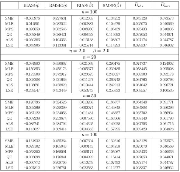
The measures Dabs and Dmax are overall measures which are useful, especially in cases of vector-valued parameters. The results of the simulation are included in Table 1.
Table 1: Simulation Results
BIAS(ηˆ) RMSE(ηˆ) BIAS(ˆ) RMSE(ˆ) Dabs Dmax η = 0.5 = 0.5
n = 20
SME -0.024024 0.162010 0.093632 0.362101 0.074604 0.123659
MLE 0.037713 0.114543 0.037520 0.259470 0.058445 0.095007
MPS -0.030877 0.093229 0.065505 0.275623 0.059303 0.092178
QE 0.000822 0.105409 0.063802 0.302417 0.061760 0.098793
ALS -0.027173 0.107205 0.065183 0.278748 0.061042 0.096721
LSE -0.050887 0.113362 0.106048 0.314732 0.063557 0.100535
n = 50
SME -0.031815 0.131082 0.041084 0.206989 0.054322 0.091703
MLE 0.013067 0.059600 0.016180 0.152725 0.034888 0.056296
MPS -0.021780 0.058514 0.027937 0.157295 0.035702 0.056934
QE -0.001809 0.063419 0.028048 0.176455 0.038140 0.061793
ALS -0.021435 0.071198 0.031587 0.162208 0.037753 0.061715
LSE -0.035907 0.077353 0.053775 0.177812 0.039429 0.064828
n = 100
SME -0.032997 0.113815 0.021172 0.140692 0.043129 0.073575
MLE 0.007276 0.041261 0.008366 0.105960 0.025070 0.040569
MPS -0.013325 0.041273 0.014491 0.107686 0.025433 0.040836
QE -0.001424 0.044210 0.015060 0.119348 0.027053 0.044071
ALS -0.015193 0.052176 0.019003 0.111465 0.027174 0.044787
LSE -0.024453 0.056690 0.032246 0.120105 0.028337 0.046932
η = 1.0 = 1.0 n = 20
SME -0.046659 0.324890 0.043934 0.301742 0.074684 0.123883
MLE 0.075426 0.229087 0.008626 0.240389 0.058445 0.095008
MPS -0.061754 0.186458 0.035088 0.246645 0.059303 0.092178
QE 0.001644 0.210818 0.028247 0.266655 0.061760 0.098793
ALS -0.054345 0.214410 0.034197 0.248942 0.061042 0.096721
LSE -0.101774 0.226725 0.070040 0.268354 0.063557 0.100535
n = 50
SME -0.063474 0.262230 0.022290 0.190649 0.054339 0.091749
MLE 0.026135 0.119200 0.005405 0.146810 0.034888 0.056296
MPS -0.043561 0.117028 0.016860 0.148854 0.035702 0.056934
QE -0.003619 0.126837 0.014269 0.166007 0.038140 0.061793
ALS -0.042870 0.142397 0.019944 0.152602 0.037753 0.061715
LSE -0.071814 0.154707 0.040568 0.162523 0.039429 0.064828
Table 1: Simulation Results(Continued)
BIAS(ηˆ) RMSE(ηˆ) BIAS(ˆ) RMSE(ˆ) Dabs Dmax n = 100
SME -0.065976 0.227631 0.012053 0.134252 0.043128 0.073573
MLE 0.014551 0.082522 0.002887 0.104679 0.025070 0.040569
MPS -0.026650 0.082546 0.008930 0.105459 0.025433 0.040836
QE -0.002849 0.088421 0.008322 0.116093 0.027053 0.044071
ALS -0.030386 0.104353 0.013138 0.108307 0.027174 0.044787
LSE -0.048906 0.113381 0.025714 0.114293 0.028337 0.046932
η = 2.0 = 2.0 n = 20
SME -0.091980 0.650662 0.021069 0.290175 0.074737 0.124002
MLE 0.150853 0.458173 -0.005677 0.239185 0.058445 0.095008
MPS -0.123508 0.372917 0.020625 0.240527 0.059303 0.092178
QE 0.003288 0.421636 0.011247 0.260748 0.061760 0.098793
ALS -0.108691 0.428820 0.019444 0.242913 0.061042 0.096721
LSE -0.203547 0.453449 0.053743 0.255333 0.063557 0.100535
n = 50
SME -0.126796 0.524525 0.013268 0.186857 0.054348 0.091771
MLE 0.052269 0.238399 0.000074 0.145848 0.034888 0.056296
MPS -0.087122 0.234056 0.011481 0.146657 0.035702 0.056934
QE -0.007238 0.253674 0.007580 0.163566 0.038140 0.061793
ALS -0.085741 0.284792 0.014325 0.149928 0.037753 0.061715
LSE -0.143627 0.309414 0.034383 0.157295 0.039429 0.064828
n = 100
SME -0.131932 0.455264 0.007604 0.132616 0.043128 0.073573
MLE 0.029102 0.165043 0.000143 0.104758 0.025070 0.040569
MPS -0.053300 0.165091 0.006171 0.105067 0.025433 0.040836
QE -0.005698 0.176841 0.004992 0.115414 0.027053 0.044071
ALS -0.060772 0.208706 0.010249 0.107493 0.027174 0.044787
LSE -0.097812 0.226761 0.022563 0.112277 0.028337 0.046932
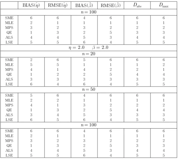
4. Summary and Concluding Remarks
From Table 1, it is observed that all the estimates seem to be consistent as the RMSE decreases when the sample size increases. The estimates appear to be asymptotically unbiased as the BIAS decreases when the sample size increases except in case of SME in estimating η. Both Dabs and Dmax decrease uniformly when the sample size increases for all cases. For a clear comparison, the rankings (smallest to largest) are given in Table 2. Here we see the performances as in the order (superior to inf erior) of MLE, MPS, QE, ALS, LSE, and SME. It should also be noted that: for smaller samples MLE in estimating η are poor; bias is the smallest in estimating η in case of QE except for n = 100, = 0.5, η = 0.5; SME
is worst by far in comparison with other estimates; ALS is better throughout in comparison with LSE. This study is beneficial in light of its inclusion of newer estimation procedures. In conclusion, MLE should be used if large sample properties are desirable and ALS should be used if the sample size is small and for computational convenience.
Table 2: Simulation Rankings
BIAS(ηˆ) RMSE(ηˆ) BIAS(ˆ) RMSE(ˆ) Dabs Dmax η = 0.5 = 0.5
n = 20
SME 2 6 5 6 6 6
MLE 5 5 1 1 1 2
MPS 4 1 4 2 2 1
QE 1 2 2 4 4 4
ALS 3 3 3 3 3 3
LSE 6 4 6 5 5 5
n = 50
SME 5 6 5 6 6 6
MLE 2 2 1 1 1 1
MPS 4 1 2 2 2 2
QE 1 3 3 4 4 4
ALS 3 4 4 3 3 3
LSE 6 5 6 5 5 5
n = 100
SME 6 6 5 6 6 6
MLE 1 1 1 1 1 1
MPS 3 2 2 2 2 2
QE 2 3 3 4 3 3
ALS 4 4 4 3 4 4
LSE 5 5 6 5 5 5
η = 1.0 = 1.0 n = 20
SME 2 6 5 6 6 6
MLE 5 5 1 1 1 2
MPS 4 1 4 2 2 1
QE 1 2 2 4 4 4
ALS 3 3 3 3 3 3
LSE 6 4 6 5 5 5
n = 50
SME 5 6 5 6 6 6
MLE 2 2 1 1 1 1
MPS 4 1 3 2 2 2
QE 1 3 2 5 4 3
ALS 3 4 4 3 3 4
LSE 6 5 6 4 5 5
Table 2: Simulation Rankings(Continued)
BIAS(ηˆ) RMSE(ηˆ) BIAS(ˆ) RMSE(ˆ) Dabs Dmax n = 100
SME 6 6 4 6 6 6
MLE 2 1 1 1 1 1
MPS 3 2 3 2 2 2
QE 1 3 2 5 3 3
ALS 4 4 5 3 4 4
LSE 5 5 6 4 5 5
η = 2.0 = 2.0 n = 20
SME 2 6 5 6 6 6
MLE 5 5 1 1 1 2
MPS 4 1 4 2 2 1
QE 1 2 2 5 4 4
ALS 3 3 3 3 3 3
LSE 6 4 6 4 5 5
n = 50
SME 5 6 4 6 6 6
MLE 2 2 1 1 1 1
MPS 4 1 3 2 2 2
QE 1 3 2 5 4 4
ALS 3 4 5 3 3 3
LSE 6 5 6 4 5 5
n = 100
SME 6 6 4 6 6 6
MLE 2 1 1 1 1 1
MPS 3 2 3 2 2 2
QE 1 3 2 5 3 3
ALS 4 4 5 3 4 4
LSE 5 5 6 4 5 5
5. Acknowledgement
The authors would like to thank the editor for facilitating the publication of the paper. The authors also would like to thank the referees for their useful comments which improved the presentation of the paper significantly.
References
1. AL-FAWZAN, M. A. Methods for estimating the parameters of the Weibull distribution. Interstat, October 2000, 1-11.
2. CASTILLO, E. and HADI, A. S. (1995). A method for estimating
parameters and quantiles of distributions of continuous random variables.
Computational Statistics & Data Analysis, 20, 421-439.
3. CHENG, R. C. H. and AMIN, N. A. K. (1983). Estimating Parameters in Continuous Univariate Distributions with a Shifted Origin. Journal of Royal Statistical Society, Series B, 45(3), 394-403.
4. CHENG, R. C. H. and ILES, T. C. (1987). Corrected Maximum
Likelihood in Non-Regular Problems. Journal of Royal Statistical Society, Series B, 49(1), 95-101.
5. ENGELHARDT, M. (1975). On simple estimation of the parameters of the Weibull or extreme-value distribution. Technometrics, 17(3), 369-374.
6. HARTER, H. L. (1965). Point and interval estimators based on order statistics for the scale parameter of a Weibull population with known shape parameter. Technometrics, 7(3), 405-422.
7. HARTER, H. L. and MOORE, A. H. (1965). Maximum likelihood estimation of the parameters of Gamma and Weibull populations from complete and from censored samples. Technometrics, 7(4), 639-643.
8. QUANDT, R. E. (1966). Old and new methods of estimation and the Pareto distribution. Metrika, 10, 55-82.
9. RANNEBY, B. (1984). The Maximum Spacing Method. An Estimation Method Related to the Maximum Likelihood Method. Scandanavian Journal of Statistics, 11, 93-112.
10. SCHMID, U. (1997). Percentile estimators for the three-parameter weibull distribution for use when all parameters are unknown.
Communications in Statistics - Theory and Methods, 26(3), 765-785.
11. SHAH, A. and GOKHALE, D. V. (1993). On Maximum Product of Spacings (MPS) Estimation for Burr XII Distributions. Communications in Statistics - Simulation and Computation. 22(3), 615-641.
12. STONE, G. C. and HEESWIJK, G. V. (1977). Parameter estimation for the Weibull distribution. IEEE Trans. on Elect. Insul., EI-12(4), 253-260.
THOMAS, D. L. (1976). Reciprocal moments of linear combinations of exponential variates. Journal of the American Statistical Association, 71, 506-512.
[ received date : Aug. 2003, accepted date : Oct. 2003 ]