†2013년 1월 30일 접수 ~ 2013년 3월 25일 심사완료
* Student, School of Mechanical and Aerospace
Engineering, Gyeongsang National University
** Regular, School of Mechanical Engineering, ERI, Gyeongsang National University
E-mail: [email protected]
Coin Drop Simulation based on Smoothed Particles Hydrodynamics
Han-bin Kang*, In-seok Pack*, Ju-han Song*, Dong-ug Lee*, Min-hyeok Park*, and Seok-soon Lee**
ABSTRACT
Smoothed Particle Hydrodynamics(SPH) method uses a grid of historical analysis and is not Lagrangian particles using the grid method. The Navier-Stokes equations were used to solve the viscous flow of the non-compressed. In this study, the numerical analysis of the three-dimensional Coin Drop Simulation using SPH method was performed, and the analysis results are compared with experimental results, and a similar behavior can be seen. The commercial program used was Abaqus/Explicit. SPH method to reduce the error by comparing the existing flow analysis or interpretation of the continuing research is needed in the future. That will enable real-time analysis of material obtained as a result of these numerical simulations similar to the actual flow phenomena, depending on the development of computer graphics technology to show visually. As a result, this method can be applied to the analysis fluid - structure interaction problems in a variety of fields.
Key Words: Smoothed Particle Hydrodynamics(SPH), Governing Equation, Kernel Function, Kernel Approximation, Particle Approximation
Symbol
: Arbitrary Function : Continuous Function : Density [] : Velocity [ ] : Internal Energy [J] : External Force [N]
: Pressure [Pa]
1. Introduction
Gridless, mesh-free continuum mechanics to solve problems and robust, can handle large deformation without difficulty that has much potential suggested by Lucy and Gingold &
Monaghan, who pioneered the SPH (Smoothed
Particle Hydrodynamics) method that was
evaluated. However, it is compared to the
possibility of the lack of consistency,
accuracy and stability of the problem,
especially at the boundaries of the defect
to be overcome.[1,2]
Increasing computation speed and the capacity of the computer, the theoretical analysis of physical phenomena is not easy to solve using numerical computer simulation techniques, though it has been actively researched. These numerical simulation techniques by experiments on a complex phenomenon that is difficult to measure the flow from the conventional to the more time-consuming and costly experiments except the difficult to measure and predict physical phenomena, have been widely used to calculate the data obtained as a result of these numerical simulation techniques and is also made possible with the advancement of computer graphics technology depending on the time closer to the actual flow and visibility, and real-time analysis can show that.
To interpret the existing flow in order to perform the numerical simulation of these phenomena, Boundary Element Method (BEM), Finite Element Method (FEM) and Finite Difference Method (FDM) are used. These methods, however, have difficulties in handling the moving contact surface of the material, the deformation of the boundary, and the free surface.
The SPH particles using a grid to solve these difficulties as a pure Lagrangian technique, started in the 1970s astrophysics sector (Gingold & Monaghan, 1977), and was applied to the free-flow of sleep (Monaghan, 1994), a low Reynolds number structure acting on wave pressure research (Gomez &
Dalrymple, 2004) to a variety of fields, including in the incompressible fluid analysis (Morris et al. 1997) have been attempted.[3-5]
2. Theory
2.1 General SPH Theory
SPH interpolation on the basis of the theory has been mainly used to solve the problem of continuum mechanics. Of the field variables at a single point through the following, ‘kernel approximation’
〈〉
′
′
′(1)
and ‘particle approximation’
≅
(2)
may be obtained from the information of the surrounding particles. Here, f is an arbitrary function, the subscript i, j is the number of particles, N is number of particles of the i particles affecting around commonly referred to as the kernel function, W having a width which is determined parameters, and h as a continuous function for each representation.
SPH expression of the basic conservation equations of continuum mechanics are as follows.
(3)
(4)
(5) General SPH approximation of the above equation represents a method as follows.
(6)
(7)
(8)
Here, ρ is density, m is the mass of the particle, U the velocity, E the internal energy, α, β in the space of tensor index, respectively. In addition to the above formula, to prevent numerical instability interpreted according to the progress of artificial viscosity, emulsification change the length of the expression, considering the strength of the material type, the EOS is added to calculate the pressure.
2.2 Governing Equation
The governing equations for inviscid flow, weakly compressible fluid continuity equation and the momentum equations of the SPH technique above are as follows.
∇
(9)
∏
∇
(10) Here, v
i, x
iindicates the location of the velocity of each particle i, ∇ is the particle i, F
iis the external force, the nuclear function represents the increase or decrease. Pressure P
i, under the assumption of weak compressibility calculated using the equation of state (12).
2.3 Kernel Function
SPH techniques play an important role in the interpretation of particles to the affected area to determine the nuclear functions. The cubic spline function was used as commonly used by Monaghan &
Lattanzio(1985) proposed in this study. This function is calculated because only particles within the spatial domain, which is the continuity equation, momentum equation (9) and (10) reducing the time it takes to calculate.
×
≤≤
≤
(11)
Where R = r/h, r is the distance between the particle and x'.[6]
2.4 Equation of State
SPH method for the flow of incompressible free surface. Pressure of the fluid can be obtained from the following equation of state (Batchelor, 1967; Monaghan, 1994).[7]
(12) Where B is a constant which is determined in accordance with the conditions, γ is a dimensionless constant, ρ
0 is the initial density.
2.5 Artificial Viscosity
At the edge of the numerical dissipation to remove the virtual viscosity used in SPH techniques, Monaghan & Gingold (1983) on the virtual viscosity Π
ijthe following equation (13) is presented.[8]
∏
∙
∙
(13)
Where c represents the speed of sound,
,
,
∙
. volumetric viscous shear and momentum conservation equations, β term and to prevent cross-contamination particles in a collision with a high Mach number, similar to the Von Neumann-Richtmyer viscosity, η α term value of numerical dissipation is a small value to avoid.
2.6 Boundary Barrier Condition
Gomez & Dalrymple (2004) proposed a staggered grid arrangement of the partition wall of the particle array as used in this study, and in order to prevent the penetration of the partition wall of the Lennard-Jones form the following equation was used.
≤
(14)
Where n
1, n
2, varying parameters in accordance with the terms of the D, r
0is the initial particle spacing.
2.7 Stability Condition of Analysis
Time increment that satisfies following two stable conditions for the analysis of stability were considered in this study.
Shao & Lo (2003) of the Courant conditional expression (15), and considering the viscous diffusion Morris et al. (1997) of the conditional expression (16) was used.[9]
≤
max
(15)
≤
(16) Where l
0is the initial particle spacing of V
maxis the maximum velocity, v the kinematic viscosity coefficient.
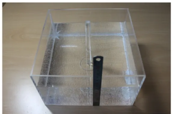
Fig. 1 Consist of Experiment Equipment
Fig. 2 Made of Arcrylic Water Tank
Fig. 3 Made of Steel Coin
3. Experiment Equipment
Experimental equipment used in this study, as shown in Fig. 1 were tank, coin and camcorders and the total was composed of three.
First tank used a 3mm thick acrylic plate,
as shown in Fig. 2. The box was manufactured
with a square perforated horizontal 200mm,
height 200mm, height of 100mm above. It is
stable to fall and when the coin falls to
the surface, φ10-acrylic pillars built in
the center of the box, serve as a guiding
craft. It was also facilitated in the tank
by attaching a 20cm cut, measuring the depth
of the coin going into the water after
shooting.
Coin outer diameter φ50 diameter φ10 ± 0.1, as shown in Fig. 3; made of steel with 1.2mm thickness using laser processing. This made the present study for the experimental program and the verification phase because was made of arbitrary size.
0.0024-per-second frame stamped, as a result, using the feature with its own slow motion, 420 frames per second were shot.
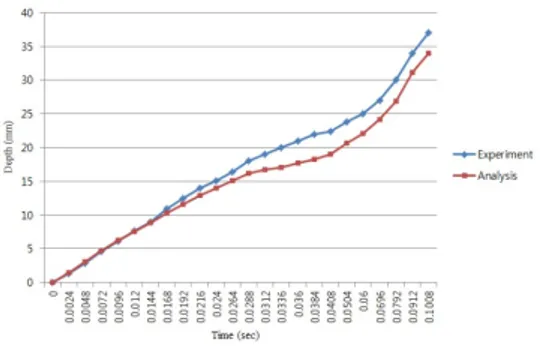
Fig. 4 Through Comparing the Experimental and Analysis Results for Graph
Fig. 5 Velocity Distribution of Analysis Result
Fig. 6 Acceleration Distribution of Analysis Result
4. Experiment & Analysis Result
Figure 4 and as the coin in the water will settle with almost similar behavior by 0.03 seconds, then the depth of the affected air in comparison. Time thereafter, but with a similar tendency can be seen the degree of tolerance. 0.03 to 0.035 seconds constant during the displacement of about 0.005, so that the uniform motion 0.03 until early linear curve appears for a short time, but the overall distribution of the graph can be seen. At interval 0.03 to 0.04 seconds the most errors occurred, namely the impact of the air gradually reduced the interval coin that is put into the water, but this time the experimental results and interpretation of the results in the error rate were largely the reason I probably interpreted in a program exactly this interval suspect is unable expressed.
Figure 5 shows the analysis results for the velocity distribution. Phenomenon occurs and the speed is drastically reduced in the early part of the almost constant or decreased slightly in the air of the affected segment. 0.04 seconds of air which is not affected since the interval can be seen that the initial rapid decrease gradually reduced, but the slope of the constant is shrinking.
Figure 6 shows the analysis results for
the acceleration distribution. After an
initial short period of time, the
acceleration increases sharply by analysis
program errors and initial conditions, but
not exactly, but failing to fully implement
the actual experimental environment seems to
be the reason.
Fig. 7 Time=0.01sec (Experiment)
Fig. 8 Time=0.02sec (Experiment)
Fig. 9 Time=0.03sec (Experiment)
Fig. 10 Time=0.04sec (Experiment)
Fig. 11 Time=0.01sec (Analysis)
Fig. 12 Time=0.02sec (Analysis)
Fig. 13 Time=0.03sec (Analysis)
Fig. 14 Time=0.04sec (Analysis)
Conclusion
When I compared the analytical results and the experimental results shows similar behavior was observed.
Interpreting time finite element grid or generate more a little more closely divided, to be supplemented in the future be able to get better results than expected.
Acknowledgments
This research was financially supported by the Ministry of Education, and National Research Foundation (NRF) through the second phase BK 21 program and the regional innovation training project and Dongnam Leading Industry Office (DLIO).
Reference
[1] L.B.Lucy, A numerical approach to the testing of the fission hypothesis,
Astronomical Journal, 1977, 82, 1013-1020.
[2] R.A.Gingold, J.J.Monaghan, Smoothed particle hydrodynamics : theory and application to nonspherical stars,
Monthly Notices of the Royal AstronomicalSociety