Introduction
A great deal of work has been done and many methods have been developed to obtain energy consumption loads for buildings. Some works (Mitalas et al., 1967, 1968) use the transfer function approach for calculating energy loads. This concept is first introduced by them using what they call room
thermal response factors (Stephenson et al., 1967).
Their procedure is as follows: the room surface temperatures and cooling or heating load are first calculated in a rigorous manner for several typical constructions. In these calculations, the components such as solar heat gain, conduction heat gain, or heat gain from lighting, equipment, and occupants are DOI:10.3796/KSFT.2011.47.2.046
The study of simplified technique compared with analytical solution method for calculating the energy consumption loads of
four houses having various wall construction
Kyu-Il H AN *
Department of Mechanical System Engineering, Pukyong National University, Busan 608-739, Korea
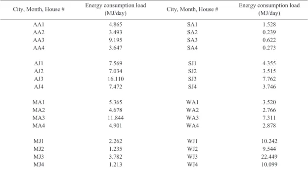
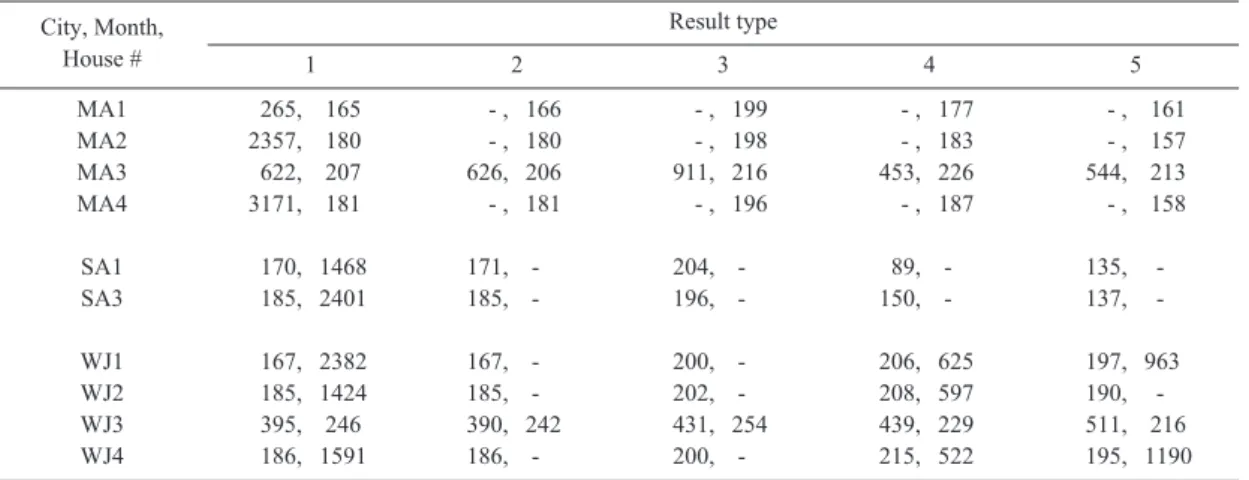
A steady-state analysis and a simple dynamic model as simplified methods are developed, and results of energy consumption loads are compared with results obtained using computer to evaluate the analytical solution. Before obtaining simplified model a mathematical model is formulated for the effect of wall mass on the thermal performance of four different houses having various wall construction. This analytical study was motivated by the experimental work of Burch et al. An analytical solution of one-dimensional, linear, partial differential equation for wall temperature profiles and room air temperatures is obtained using the Laplace transform method. Typical Meteorological Year data are processed to yield hourly average monthly values. This study is conducted using weather data from four different locations in the United States:
Albuquerque, New mexico; Miami, Florida; Santa Maria, California; and Washington D.C. for both winter and summer conditions. The steady state analysis that does not include the effect of thermal mass can provide an accurate estimate of energy consumption in most cases except for houses #2 and #4 in mild weather areas. This result shows that there is an effect of mass on the thermal performance of heavily constructed house in mild weather conditions. The simple dynamic model is applicable for high cycling rates and accurate values of inside wall temperature and ambient air temperature.
Keywords: Steady state, Energy consumption load, Thermal mass, One-dimensional, Thermal performance
* Corresponding author: [email protected], Tel: 82-51-629-6194, Fax: 82-51-629-6188
simulated by pulses of unit strength. The transfer functions are then calculated as numerical constants which represent the cooling or heating load excitation pulses corresponding to the input excitation pulses.
The method of Mitalas (1968) assumes that heat flow through building elements is one-dimensional, i.e. effects of room corners or other irregularities are ignored, and that room air temperature is uniform throughout the room. This method can handle periodic or non-periodic ambient conditions and variable surface heat transfer coefficients.
Peavy et al. (1973) and Kusuda (1976) also use a response factor method for their computer program to calculate building loads. It is concluded that a combination of mass in walls and roof facing the interior with insulation placed on the outer surfaces of a building is very effective in reducing and controlling the variation of the indoor air tempera- ture. Kusuda conducts a computer program for prediction of dynamic thermal and energy loads of buildings is presented. Those results are compared with experimental results obtained from laboratory measurements made on an experimental building.
Kusuda (1981) compares computer simulation results with the method developed by ASHRAE’s Technical Committee on energy calculation.
However, transient effects brought about through controls (time dependent thermostat and fan switch setting) are not included, and thermal storage effects of the building components and dead-band control also are not simulated.
A finite differences method is used by Cuplinskas (1977) for thermal response calculations. The finite differences method is frequently used to solve more complex dynamic problems in heat transfer than can be handled by analytical methods. His proposed method is not meant as a substitute for the more
elaborate methods, but as an alternative simplified solution that is easily understood and programmed by engineers.
A degree-day method is used by Webster (1985) for small buildings. The method is based on the principle that the energy requirement for space heating is primarily dependent on the difference in temperature between indoors and outdoors.
In Jones et al. (1982), an evaluation is made of the thermal performance of 4 double-envelope house built in Middletown, Rhode Island. It is concluded that the low heating energy needs of the house are due primarily to the excellent insulative value of the double shell. The double-shell construction of the house results in very low air infiltration, even on windy days.
Similar results for investigating which construction materials consume less energy under varying climatic conditions are obtained by Burch et al. (1984). His group recently conducted experiments on six test buildings in Gaithersburg, MO. These buildings were instrumented to measure heating and cooling loads, and indoor comfort.
They focus on the effect of different construction materials in determining the energy consumption load.
All of these studies are deficient in one or more ways. The experimental studies exhibit a very small savings due to mass of the same magnitude as the effect of solar radiation absorbed by and transmitted through the walls. The analytical studies do not include a realistic model of the energy plant.
The main purpose of this study is to develop a
simplified method from a rigorous mathematical
basis to analyze the energy consumption load and
calculating the cycling time corresponding to on-
off controller and to compare the results with the
analytical solution.
Theoretical formulation for analytical solution
The formulation of an analytical method for obtaining wall temperature profile, room air temperature, and energy consumption load is presented. Four of the six houses studied by Burch et al. are modelled. Each test house is a 6.1m by 6.1m by 2.3m one-room house. The houses have identical floor plans and orientations, and are identical except for wall construction, which is as follows: insulated lightweight wood frame;
insulated masonry with outside mass; uninsulated masonry; and insulated masonry with inside mass.
The details of the wall construction for each of the four houses are presented in Table 1.
Weather data for four cities in the United States are used in this study. Twenty-four discrete data points calculated from TMY (Typical Meteorologi- cal Year) weather data files (1998) are converted to continuous form via a Fast Fourier Transform (Brigham, 2004). Each house is modelled by a single homogeneous wall and an air node.
The system is considered as one-dimensional.
The heat transfers in the y and z directions are assumed to be negligible, and the heat flow occurs principally in the direction perpendicular to the surface of the wall (x-direction). Neglect of heat flow in the y and z directions should not significantly affect the applicability of the solution (Myers, 2001).
Under this study there is no heat generation within the wall, and the energy balance, after some manipulation, yields:
∂
2T/∂x
2〓(1/a)∂T/∂t (1)
Two corresponding boundary conditions to the above linear, second-order, partial differential equation are:
-k∂T/∂x (x〓0)〓âS*+h e (T ∞ -T 0 ) (2)
-k∂T/∂x (x〓L)〓-h i (T A -T L ) (3) The initial condition for the wall temperature is expressed in polynomial form as:
T (x, 0) 〓 n〓0 ∑
4a n x
n(4) The energy balance for the room air temperature including heat transfer from the inside surface of the wall, infiltration loss, and auxiliary heat input Q, is:
C A dT A /dt 〓-h i A (T A -T L ) -C A ′I (A A -T ∞ ) +Q (5) Table 1. Wall construction types
House #1 : insulated lightweight wood frame 13mm (0.5 in) gypsum board
0.05mm (0.002 in) polyethylene film
50×100 mm (2×4 in) studs placed 410 mm (16 in) o.c.
with R-11 16 mm (5/8 in) exterior plywood House #2 : insulated masonry (outside mass) 13mm (0.5 in) gypsum board
0.05mm (0.002 in) polyethylene film
51 mm (2 in) thick extruded polystyrene insulation placed between 38 mm (1 -1/2 in) wide wood furring strips placed 610 mm (24 in) o.c.
6.4 mm (1/4 in) air space
100mm (4 in) 2-core hollow concrete block 1680 kg/m3 (105 lb/ft3)
100 mm (4 in) face brick House #3 : uninsulated masonry 13mm (0.5 in) gypsum board 0.05mm (0.002 in) polyethylene film
20 mm (3/4 in) air space created by 50×20 mm (2×3/4 in) furring strips placed 410 mm (16 in) o.c.
200 mm (8 in) 2 -core hollow concrete block 1680 kg/m
3(105 lb/ft3)
House #4 : insulated masonry (inside mass) 13 mm (0.5 in) plaster
200 mm (8 in) 2-core hollow concrete block 1680 kg/m
3(105 lb/ft3)
89mm (3 -1/2 in) perlite insulation in space between block and brick
100 mm (4 in) face brick
C A 〓(rC v ) A V A (6)
C A ′ 〓(rC p ) A V A (7)
I ′〓C A ′ I /C A (8)
The parameters, h i , h e , C A , C A ′ and I are assumed constant.
The corresponding initial condition to equation (5) is as follows:
T A (0) 〓T i (9)
Weather data for four cities in the United States are used in this study. Those cities under study are Albuquerque, NM; Miami, FL; Santa Maria, CA;
and Washington, D.C. Two of the cities, Albuquerque and Washington D.C., have four distinct seasons, while Santa Maria experiences mild weather conditions year round. Miami weather is the hottest of the four cities studied, and houses need to be cooled nearly year round. TMY (Typical Meteorological Year) weather data files are used to obtain hourly values of the solar flux and ambient temperature.
The weather data input to the analytical model is finally represented in the following form:
S*(t) 〓b 0 + ∑
11i〓1 [b i cos (w i t +F i ) +c i sin(w i t +F i )]
(10) T ∞ (t) 〓d 0 + ∑
11i〓1 [d i cos (w i t +F i ) +e i sin(w i t +F i )]
(11) where b 0 is the DC component of the solar flux and d 0 is the DC component of the ambient temperature.
The Laplace transform solution technique (Kreyszig, 2006) is successfully applied to the problem under study, and the inversion from the Laplace domain to the time domain is accomplished using the complex inversion theorem using
Bromwich contour (Carslaw et al., 1959).
The form of the wall temperature as a function of time is:
T (x,t) 〓 m〓1 ∑
∞[(A m /C m )EXP ( -ah
2m t) cos (h m x)
+(B m /C m )EXP ( -ah
2m t) sin (h m x)]
+a 0 +a 1 x+a 2 x
2+a 3 x
3+a 4 x
4+2aa 2 t
+12a
2a 4 t
2+6aa 3 xt+12aa 4 x
2t
+(1/2)[(N 1 /D)(t
2+tx
2/a+x
4/(12a
2))
+(N 1 ′ /D)(2t +x
2/a)+N 1 ″/D-D″N 1 /D
2-(2D′ /D
2) [(t +x
2/(2a))N 1 +N 1 ′ ]
+2D′
2N 1 /D
3+(N 2 /D)(t
2x+tx
3/(3a)
+x
5/(60a
2))+(N 2 ′ /D)(2tx+x
3/(3a))
+N 2 ″x/D-D″N 2 x/D
2-(2D′ /D
2)[(tx
+x
3/(6a ))N 2 +N 2 ′ x] +2D′
2N 2 x/D
3]
+ ∑
11i〓1 [x 1i (x) cos (w i t) +x 2i (x) sin (w i t)]
(12) The form of the room air temperature as a function of time is:
T A (t) 〓 m〓1 ∑
∞[(A m /C m )Mcos (h m L) EXP ( -ah
2m t)
+(B m /D m ) Msin (h m L)EXP (-ah
2m t)
+((c 32 +c 36 )/c 33 -c 39 +c 42 +T i ) EXP (-bt)+(1/2)[F 6 /F 1 -(F 4 D″+2F 5 F 2 )/(F 1 )
2+2F 4 (F 2 )
2+F 9 /F 1 -(F 7 F 3 +2F 8 F 2 )/(F 1 )
2+2F 7 (F 2 )
2/(F 1 )
3]
+ ∑
11i〓1 [(x 3i +F 10 )cos (w i t)+(x 4i +F 11 ) sin (w i t)]
+(Ma
*/b-Mc
*/b
2)t+Mc
*t
2/(2b)+c
39(13) where h m is the m
throot of the characteristic equation:
tan (Lh m )〓[-h m (c 14 s m +c 15 )]/[c 16 s
2m +c 17 s m +c 18 ] (14) Attention is now turned to the process of switching modes, e.g. from heating to no heating.
In the case of on-off control, this occurs when the
room air temperature exceeds the dead band. This
effects a partitioning in time, shown in Fig. 1, as
region I and region ll, when the heating system is
“off”and“on”, respectively.
Now we will discuss the steps used to obtain the times mentioned above for on-off control. We will illustrate the process during the heating season.
First, the weather data, equations (10) and (11), are rearranged as follows:
S
*〓b 0 + ∑
11i〓1 [b i cos [w i (t+t
*)]+c i sin[w i (t+t
*)]]
(15)
T ∞ 〓d 0 + ∑
11i〓1 [d i cos [w i (t +t
*)] +e i sin[w i (t +t
*)]]
(16) where t
*is time at which the controller function changes.
In the first region:
1) Take initial conditions for the wall temperature,
T w (x,t
*), and the room air temperature, T i . 2) Let Q and t
*be zero. This arbitrarily implies
no heating, and results in temperature decay as shown in Fig. 1.
3) Obtain t 1 using a bisection method.
In the second region:
1) Calculate a new initial condition by evaluating the solution for T w (x, t
*) and calculating coefficients a 0 to a 4 as presented in equation (4). The new initial state for T A 〓(-DB).
2) Let Q〓Q teating .
3) Take new weather data which is the original weather data shifted by w i t 1 (i.e. w i t
*).
4) Obtain t 2 using a bisection method.
The process repeats until a complete daily cycle is exhausted. At the end of a day, the state of the system is compared with that at the beginning of the day. If the states (temperature profile in the wall and room air temperature) agree to within a specified small tolerance, the solution has converged. If not, the daily cycle is repeated with new initial conditions equal to the present state of the system. Note that whenever the auxiliary energy source switches, new t
*(cumulative time, i.e.: t 1 +t 2 +t 3 +…) should be used for the weather equations, (15) and (16).
After obtaining all times for switchover points, a graph of T A versus time for a 24 hour period is processed, and inspected for consistency. In the case of heating, T A is not supposed to be below (-DB) in Fig. 1. T A below (-DB) means that the switchover point is missed, and the times are recalculated after readjusting the input data points for the bisection method.
Total heating or cooling time per day is obtained by summing the times during which the auxiliary energy is on. Then, heating/cooling loads per day can be calculated.
Fig. 1. Room air temperature trajectory and auxiliary energy input.
Case of cooling Case of heatng Auxiliary enevgy
t
1t
2t
3t
4t
t
t
Ⅰ Ⅱ Ⅰ Ⅱ
+DB
-DB
+Q
0
-Q
+Q
0
-Q
Ti
Ts
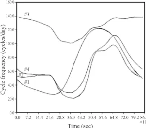
Formal calculation of cycle rate can be obtained as follows:
f n 〓86400/(Dt n ) (17)
where f n is the cycle frequency (cycles/day) and Dt n
is the time interval for one cycle (secs/cycle) as shown in Fig. 2. Results for all four houses are shown in Fig. 3 for Miami (cooling) and Fig. 4 for Washington D.C. (heating). Frequent cycling exists in August in Miami for house #3. House #3 also shows the lowest variation in cycle rate compared with the other insulated houses. House #1 shows the highest variation in cycle rate.
Simplified technique
Two models are presented to approximate the energy consumption load and to investigate the cycling rate. Zero capacitance model is used for calculating the energy consumption approximately and simplified dynamic model is used for investigating the cycling rate.
The detailed results using accurate analytical solution require a large number of complex and repetitive calculations. Coding a computer program and using it is time-consuming and a boring job. It is desirable, therefore, for the engineer or building designer to have a method to quickly estimate the energy load for buildings .
A steady-state analysis is introduced to approximate the load. As shown in Fig. 5, ambient temperature and solar radiation can be combined in the form of the sol-air temperature in ASHRAE handbook (1982) to simplify the analysis. The sol- air temperature is that outdoor air temperature which, in the absence of all radiative exchange, gives the same rate of heat input to the surface of the wall as exists with the actual incident solar radiation, radiant energy exchange with the sky and other outdoor surroundings, and convective heat Fig. 4. Cycle frequency vs. time (Washington D.C.,
January).
160.0 140.0 120.0 100.0 80.0 60.0 40.0 20.0
0.0 0.0 7.2 14.4 21.6 28.8 36.0 43.2 50.4 57.6 64.8 72.0 79.2 86.4
C yc le f re qu en cy ( cy cl es /d ay )
Time (sec)
Fig. 3. Cycle frequency vs. time (Miami, August).
160.0 140.0 120.0 100.0 80.0 60.0 40.0 20.0
0.0 0.0 7.2 14.4 21.6 28.8 36.0 43.2 50.4 57.6 64.8 72.0 79.2 86.4
×10
3×10
3#3
#3
#4
#1
#4
#2
#2
#1
C yc le f re qu en cy ( cy cl es /d ay )
Time (sec)
Fig. 2. Calculation method for cycle frequency.
86400 f
1= _____ (cycles/day)
Dt
186400 f
2= _____ (cycles/day)
Dt
2Dt
1Dt
2Dt
3t
1t
2t
3T
A+DB
-DB
t
exchange with the outdoor air. It is represented as follows:
T sol-air +T ∞ +âS/h e -eDR/h e (18)
where e is hemispherical emittance of the surface, and DR is the difference between the long wave radiation incident on the surface from the sky and surroundings, and the radiation emitted by a blackbody at ambient temperature.
It is difficult to determine an accurate value of DR, since vertical surfaces receive long wave radiation from the ground and surrounding buildings as well as from the sky. When the solar radiation intensity is high, surfaces of terrestrial objects usually have a higher temperature than the ambient air temperature; thus, their long wave radiation compensates to some extent for the sky′ s low emittance. Also, during the day, the solar exchange typically dwarfs the long wave radiative exchange. Therefore, it is reasonable to assume DR
〓0 for vertical surfaces. Equation (18) can then be rewritten as:
T sol-air 〓T ∞ +âS/h e (19)
Thus, the steady-state heat flow for the building maybe calculated as:
______ __
Q S 〓±UA (T sol-air -T
*A )+C A ′ I (T ∞ -T
*A ) (+ sign: cooling, -sign: heating) (20)
U 〓1/(1/h e +L/k+1/h i ) (21)
where U is overall heat transfer coefficient, ___
T sol-air ____ , ___ T ∞ and T
*A are the average sol-air temperature, ambient temperature and room air temperature, respectively.
Here, heat flow by infiltration is added to Q in equation (20). Two average room air temperatures are used for T
*A : one is the set-point temperature T s , which is 22, and the other is the average room air temperature from the computer output in the case of the on-off controller, ___
T A .
The study now turns its attention to the simplified dynamic model for investigating the cycling rate. In this model, T L is assumed to be known, and equation (5).
Equation (5) is rearranged as follows:
dT A /dt +(a
*+b
*)T A 〓a
*T L +b
*T ∞ +c
*(22) where:
a
*〓h i A/C A (23)
b
*〓C A ′ I/C A (24)
c
*〓Q/C A (25)
Equation (22) becomes:
dT A /dt+B
*T A 〓A
*(26)
when:
A
*〓a
*T L +b
*T ∞ +c
*(27)
B
*〓a
*+b
*(28)
A
*is assumed constant, as T L and T ∞ are nearly constant for a short cycle period.
Equation (26) is solved subject to initial conditions over the cycle interval. There are two initial conditions to be considered: one is the room air temperature, T A , at the upper bound of the Fig. 5. Sol-air temperature for steady-state analysis.
âs Wall
Wall T
∞T
sol-air1/h
ex=0
x=0
x=L
x=L 1/h
iL/k
1/h
eL/k 1/h
iT
AT
Adeadband, the other is T A at the lower bound of the deadband. For convenience, let T A at the upper bound be T
+A , and T A at the lower bound be T
-A , respectively. c
*becomes Q/C A or zero, depending on whether the auxiliary energy source is on or off.
Solutions to equation (26) for the heating case are shown below:
1) For heating cycle,
T A 〓(T
-A -A
*/B
*) EXP ( -B
*t) +A
*/B
*(29) 2) For no-heating cycle,
T A 〓(T
+A -A
*/B
*) EXP (-B
*t)+A
*/B
*(30) No-heating cycle implies that the room air temperature variation in the case of no auxiliary energy (Q 〓0). Solutions to equation (26) for the cooling case are reversed.
Table 2. Average temperatures and energy consumption loads for steady-state (T
*A〓T
s) City, Month, House #
____T
sol-air____
T
0____