노드 모니터링에 의한 효율적인 LDPC 디코딩 알고리듬
서희종*
Efficient LDPC Decoding Algorithm Using Node Monitoring
Hee-Jong Suh
*요 약
본 논문에서는 노드 모니터링(NM)과 Piecewise Linear Function Approximation(: NP)을 사용하여 LDPC 디 코딩 알고리듬의 계산복잡도를 감소시키는 알고리듬을 제안한다. 이 알고리듬은 기존의 알고리듬보다도 더 효율 적이다. 제안된 알고리즘이 기존의 방법보다도 개선되었다는 것을 확인하기 위해서 모의실험을 하였다. 실험결과, 제안된 알고리즘의 계산은 기존의 방법에 비해 약 20 % 향상되었음을 확인하였다.
ABSTRACT
In this paper, we proposed an efficient algorithm using Node monitoring (NM) and Piecewise Linear Function Approximation(: NP) for reducing the complexity of LDPC code decoding. Proposed NM algorithm is based on a new node-threshold method together with message passing algorithm. Piecewise linear function approximation is used to reduce the complexity of the algorithm. This new algorithm was simulated in order to verify its efficiency. Complexity of our new NM algorithm is improved to about 20% compared with well-known methods according to simulation results.
키워드
LDPC Codes, Node Monitoring, Node-Threshold, Piecewise Linear Function Approximation LDPC 코드, 노드 모니터링, 노드-임계치, 구분적 선형함수 근사
* 교신저자: 전남대학교 전자통신공학과 ㆍ접 수 일 : 2015. 10. 02
ㆍ수정완료일 : 2015. 11. 13 ㆍ게재확정일 : 2015. 11. 23
ㆍReceived : Oct. 02, 2015, Revised : Nov. 13, 2015, Accepted : Nov. 23, 2015 ㆍCorresponding Author : Hee-jong Suh
Dept. of Electronic Communication Engineering, Chonnam National University, Email : [email protected]
Ⅰ. Introduction
Low-density parity-check (LDPC) codes were first proposed by Gallager in his doctoral dissertation [1] and were forgotten for several decades. The study of LDPC codes was resurrected in the mid-1990s because of its good performance and lower decoding complexity. LDPC codes are linear block codes which are falling only 0.04dB short of the Shannon limit [2].
LDPC codes algorithm has two parts, which are encoding and decoding. Its encoding is very easy, but its decoding is more complicated. Decoding process of the LDPC code takes much time with the existing algorithms [1-3].
There are three approaches existing to reduce the
complexity of LDPC decoding, which are to simplify
the computation of the decoder, reduce the number
of iterations of the decoder and diminish the
messages of the iterations. In this approaches, there
are many algorithms, such as the massage passing algorithm (MPA) [2],[8], the min-sum algorithm [4], the various scheduling techniques [5], the forced convergence method [3],[6] and the bit-level stopping method [7]. The MPA algorithm is known as most effective methods among the well-known methods [6].
In this paper, we propose a node monitoring (NM) algorithm. This method is a new one on reducing the decoding complexity, which is different from the other methods because it uses two monitoring vectors to monitor all the variable nodes and check nodes. For initialization the two vectors are filled with zeros. Some nodes are steady enough in case that these nodes achieve some node-threshold, at this case the vector for these nodes will stop receiving and updating process of these nodes. Proposed algorithm uses a new method and it only monitors the check nodes instead of monitoring both the check and variable nodes.
Although it does not monitor the variable nodes, it has the same performance in monitoring the messages of the check and variable nodes. But, this will finally reduce the complexity of the decoding process. The piecewise linear function approximation [9] is a good way to reduce the function that is used in the program of the node monitoring algorithm.
To verify the efficiency of proposed algorithm, we did simulations. Then, because the MPA algorithm is known as the most effective methods among the well-known methods, we did comparing with proposed NP algorithm only with the MPA algorithm. With this comparison, we could got the conclusion that NP algorithm is more efficient method than previous known methods. Therefore, we knew our algorithm is most efficient one among the well known methods. Its efficiency was about 20% improvement.
This paper is organized as follows. Section II gives the background of the LDPC code. And
Section III introduces a new decoding algorithm of the LDPC codes and the piecewise linear function approximation. In Section IV there are the results of the simulation of the algorithm. Conclusion is Section V. References are next.
Ⅱ. Related Algorithm and Problem
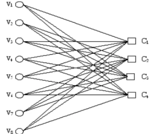
There are two types LDPC codes, regular LDPC codes and irregular LDPC codes, which can be represented by a Tanner graph with N variable nodes on the left (representing the bits of the code word) and M check nodes on the right (representing the parity checks constraints).
Fig. 1 is a Tanner graph of a block length 8 (3, 6). Nodes on the left hand side in Fig. 1 represent the code bits; nodes on the right hand side represent the parity check constraints. Throughout the decoding process, the nodes exchange messages
and
over the edges of the graph.
2.1 Standard brief propagation (BP) algorithm for iterative decoding of LDPC codes
We introduce the message passing algorithm (MPA), the most popular decoding algorithm [2], to make a our algorithm for the LDPC code decoding.
Fig. 1 Tanner graph of a block length 8 (3,6) regular
LDPC code
We suppose a regular binary ( , ) (
,
) LDPC code C is used for error control over an AWGN channel with a mean of zero and power spectral density
, and assume BPSK signals with unit energy, which maps a code word
⋯
into a transmitted sequence
⋯
, according to
, for
⋯ and
or
. If
is a code word in C, and
is the corresponding transmitted sequence, then the received sequence is
, with
, where for ≦ ≦ ,
is Gaussian random variables with a mean of zero and variance
. Let
be the parity check matrix which defines an LDPC code. We denote the set of bits that participate in check by
and the set of checks in which bit participates as
. And we denote as the set out of bit , and as the set out of check
. In order to explain the iterative decoding, we define the following notations with the th iteration:
•
: The log-likelihood ratio (LLR) of bit which is from the channel output
. In belief propagation decoding, we initially set
.
•
: The LLR of bit that check node m sends to bit node .
•
: The LLR of bit n that bit node sends to check node .
•
: The posteriori LLR of bit .
The standard belief propagation algorithm is carried out as follows [5]:
Initialization: Set = 0, and the maximum number of iteration to
. For all m, n, set
,
.
Step 1: (i) check-node update: for ≦ ≦ and each ∈ :
tanh
′∈
tanh
′ (1)
(ii) bit-node update: for ≦ ≦ and each
∈ :
′∈
′(2)
∈
(3)
Step 2: Hard decision and stopping criterion test:
(i) Create
in which
if
, and
if
≧ .
(ii) If ⋅
or
, stop the decoding iteration and go to Step 3. Otherwise set and go to Step 1.
Step 3: Output
as the decoded code word.
2.2 The complexity reducing problem
The standard belief propagation algorithm for iterative decoding of LDPC codes has about two problems. First, for both the check-to-bit messages and bit-to-check messages, the more independent information is used to update the messages, the more reliable they become. Iteration of the standard two steps implementation of the belief propagation algorithm uses all values
′ computed at the previous iteration in (1). However certain values
′could already be computed based on a partial computation of the values
obtained from (2), and then be used instead of
′ in (1) to compute the remaining values
.
So, if we use certain values
′to compute a
partial values
, then we can reduce the
complexity. Second, during the iterative decoding,
the fact is that a large number of variable nodes
converge to a strong belief after very few iterations,
i.e., these bits have already been reliably decoded
and we can skip updating their messages in subsequent iterations. If we have some ways to decide whether a node should update massage at a given iteration, then we also can reduce the complexity of the decoding process.
Ⅲ. Node Monitoring Algorithm and Piecewise Linear Function Approximation
For the two problems we described above, we introduce a decoding method based on the node monitoring algorithm. Most of the variable nodes achieve a stable state after very few iterations, barely to change the bit that it represents. So decoder could skip updating their messages in subsequent iterations. Node monitoring algorithm uses this phenomenon to reduce the complexity of the decoding. It updates messages only that instable nodes send at some iteration. In order to describe the degree of some nodes that have achieved a certain stable state, we define the "aggregate messages"
for each variable node as follows:
∈
(4)
Checking
against the node-thresholds
will find the nodes that are stable.
is the confidence of the variable node to be in state 0 or 1, and the bigger
is the more stable variable node is. Now, we introduce the node monitoring algorithm in detail. Suppose a decoding system dealing with LDPC codes. First, we define two vectors to store the state of check nodes and variable nodes, respectively. They are deactivated-v and deactivated-c. For initialization, deactivated vectors are filled with zeros. Then the variable nodes get the information bits, and compute the value
. And they send these values as messages to their neighbor check nodes. When their neighbor check nodes receive these messages, the
check nodes begin to compute their messages
and send them to variable nodes. Now, two kinds of nodes have finished their first message sending process. Variable nodes begin a deciding program to decide whether continue the next iteration or not. At this time, the variable nodes also compute
to compare with the node-threshold
. If it is bigger than the
, the element in deactivated-v to this node will change to 1 from 0. It is a flag that represents a stable node at that iteration. Then decoder checks each check nodes whether its neighbor variable nodes are all stable. If they are all in stable state, the element in deactivated-c to this node will change to 1 from 0. And this check node will not send the message to its neighbors, because its neighbors are all in stable state. But even if one of its neighbors is instable, the element in deactivated-c will still be 0, and all its neighbor variable nodes will be reactivated by resuming their elements to 0 again in deactivated-v. Then begin the new iteration just as above except that check the deactivate vector before sending the messages.
If the element for a node is 1, then skip this node’s message sending.
Piecewise linear function approximation is used to reduce the function of tanh . The function of tanh is not a linear function, so it will cost much time to compute its value. First we can write the equation (1) in another way: separate Piecewise linear function approximation is used to reduce the function of tanh . The function of tanh is not a linear function, so it will cost much time to compute its value. First we can write the equation (1) in another way: separate
to
(5)
we then have
′∈
′∙
′∈
′ (6)
Where we have
logtanh
log
(7)
The function of
is fairly well behaved, and .
But,
is not a linear function. So we use Piecewise linear function
to get an approximation of
and the complexity can thus be reduced for more. It is showed in Fig. 2.
What we have introduced above is the node monitoring algorithm. It reduces the complexity of the decoding process, but barely brings out degradation of the bit error rate(: BER) and the frame error rate (: FER) performance.
Fig. 2 The transfer function
used in check node calculations and the piecewise linear
approximation of it.
Ⅳ. Simulation Results
We simulated with a (3, 6) regular LDPC code with a block-length of 2000 bits and rate
=0.5.
Fig. 3 shows the bit error performance of three kinds of decoding algorithm for comparison. It is
easy to see that the performance of the Combination of Node Monitoring Algorithm and Piecewise Linear Function Approximation algorithm(: NM-PW) is much better.
0.2 0.3 0.4 0.5 0.6 0.7 0.8 0.9 1 1.1 1.2
5 4 3 2 1
Bit Error Rate
Eb/No (dB)
MPA F (x) F 1(x)
Fig. 3 Bit error performance of the LDPC code with a block-length of 2000 bits.
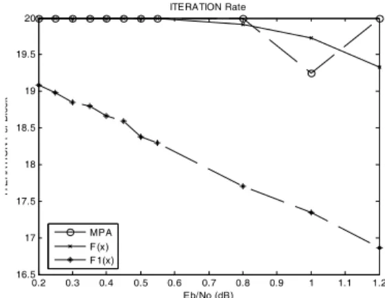
0.2 0.3 0.4 0.5 0.6 0.7 0.8 0.9 1 1.1 1.2
16.5 17 17.5 18 18.5 19 19.5
20 ITERATION Rate
ITERATION Per Block
Eb/No (dB) MPA
F (x) F 1(x)
Fig. 4 Frame error performance of the LDPC code with a block-length of 2000 bits.
Fig. 4 shows the frame error performance of
three kinds of decoding algorithm for comparison. It
is easy to see that the performance of the
Combination of Node Monitoring Algorithm and
Piecewise Linear
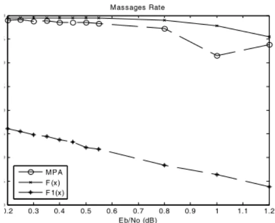
0.2 0.3 0.4 0.5 0.6 0.7 0.8 0.9 1 1.1 1.2 0
5 0 5 0 5 0 5
0 Massages Rate
Eb/No (dB) MPA
F (x) F 1(x)
Fig. 5 Messages per bit of the LDPC code with a block-length of 2000 bits.
0.2 0.3 0.4 0.5 0.6 0.7 0.8 0.9 1 1.1 1.2
-3 -2 -1
0 Frame Error Rate
Eb/No (dB)
MPA F (x) F 1(x)
Fig. 6 Iterations per block of the LDPC code with a block-length of 2000 bits.
Function Approximation algorithm (NM-PW) is performed better results too. Fig. 5 shows the Messages per bit of three kinds of decoding algorithm for comparison. It is easy to see that the complexity of the Combination of Node Monitoring Algorithm and Piecewise Linear Function Approximation algorithm (NM-PW) is about 80% of the other two. Fig. 6 shows the Iterations per block of three kinds of decoding algorithm for comparison.
As we can see from the graph, the iterations of the Combination of the Node Monitoring Algorithm and Piecewise Linear Function Approximation algorithm (NM-PW) is less than the other two.
Ⅴ. Conclusion
We have proposed a Combination of Node Monitoring Algorithm and Piecewise Linear Function Approximation algorithm (NP) to reduce the complexity of the LDPC decoding. With the simulation, we could see its better performance than existing well-known methods.
So, we can conclude that this method is the best way to reduce efficiently the complexity of the decoder. But we must endeavor in order to achieve a more practical node monitoring decoder for LDPC codes. And we must try to make more improvement to get better performance.
References
[1] C. Park, O. Kwon, and S. Yun, “New SNR Estimation Algorithm using Preamble and Performance Analysis,” Conf. of the Korea Institute of Building Construction, Seoul, Korea, Apr. 2007, pp. 93-96.
[2] S. Park, J. Lee, J. Song, and K. Oh, “RFID Technology Application in Construction Material Management Process,” Conf. of the Architectural Institute of Korea, Gwangju, Korea, Oct. 2008, pp. 593-596.
[3] J. Lee, J. Song, and K. Oh, “A Study on Developing a Context - Aware Scenario for the RFID Application of the Information Management on the Construction Materials,” J.
of the Architectural Institute of Korea, vol. 25, no.
3, 2009, pp. 111-118.
[4] IEC 61511-1, “Functional safety-safety instrumented systems for the process industry sector,” IEC, Geneva, Switzerland, Jan. 2003.
[5] IEC 61025, “Fault tree analysis(FTA),” IEC, Geneva, Switzerland, Dec. 2006.
[6] K. Chung, “Diagnosis of power supply by
analysis of chaotic nonlinear dynamics,” J. of
the Korea Institute of Electronic Communication
Sciences, vol. 9, no. 7, 2014, pp. 753-759.
[7] H. Shin, “Development of constant current SMPS for LED Lighting,” J. of the Korea Institute of Electronic Communication Sciences, vol. 10, no. 1, 2015, pp. 111-116.
[8] Y. Jeong, “A study on control of generators based on SMPS,” J. of the Korea Institute of Electronic Communication Sciences, vol. 7, no.
1, 2012, pp. 107-115.
[9] H. Shin, “Design of LED Driving SMPS for Large Traffic Signal Lamp,” J. of the Korea Institute of Electronic Communication Sciences, vol. 4, no. 2, 2009, pp. 123-129.
저자 소개
서희종(Hee-Jong Suh)