Article
http://dx.doi.org/10.4217/OPR.2015.37.4.333
Ocean and Polar Research
December 2015Physical Parameter Measurement and Theoretical Target Strength Estimation of Juvenile Cod ( Gadus macrocephalus)
Iqbal Ali Husni1, Bo-Kyu Hwang2*, Hyeon-Ok Shin3, and Min-Son Kim2
1Department of Fisheries Physics, Graduate School, Pukyong National University Busan 48513, Korea
2Department of Marine Science and Production, College of Ocean Science and Technology, Kunsan National University, Kunsan 54150, Korea
3Division of Marine Production System Management, College of Fisheries Science, Pukyong National University, Busan 48513, Korea
Abstract : The contrast (fish body to medium ratio) of density and sound speed were measured to estimate acoustic scattering from small juvenile cod (Gadus macrocephalus) with the Kirchhoff-Ray Mode back- scatter model. The density contrast was measured by the density-bottle method and the sound speed con- trast was estimated by the time of flight method. The results revealed that the measured density contrasts of juvenile cod varied between 1.003 and 1.029 (mean = 1.014, S.D. = 0.01). On the other hand, sound speed contrasts varied between 1.039 and 1.041 (mean = 1.041, S.D. = 0.001). The relationship between averaged target strength (TS) and total length (TL) established by the model were <TS38kHz> = 20log(TL)− 68.8 and
<TS120kHz> = 20log(TL)− 69.4, respectively.
Key words : density contrast, sound speed contrast, target strength, juvenile cod, Kirchhoff-Ray Mode backscatter model
1. Introduction
The Pacific cod, Gadus macrocephalus, is mainly found along the continental shelf and upper slopes of the North Pacific Ocean, from the Yellow Sea to the Bering Strait, along the Aleutian Islands. It is one of the most important commercial species in several countries, including Korea (Kim et al. 2010). Juvenile cod is a prospective recruitment, because they will return to the spawning area after growing up as their instinct in the certain season. Therefore, it is important to estimate the abundance of cod especially juvenile-stage to manage the abundance as well as to predict it.
Hydro-acoustic is a popular method to get the information on the fish abundance estimation effectively and efficiently.
And this technique has become increasingly sophisticated
and useful over the years (Simmonds and MacLennan 2005). In acoustic surveys, a quantitative echo sounder provides reflections from a fish school at various echo intensities. Field application of acoustic methods to estimate animal abundance requires information on the acoustic size, target strength or back scattering cross section of individual organisms (MacLennan 1990). This acoustic reflection is converted to quantitative data using the Target Strength (TS). It is a key quantity in the acoustic assessment of fish abundance (Foote 1987).
Acoustic scattering from fish generally could be estimated by two methods. Dual and Split-beam echo sounder used to measure TS if the target is not too small in comparison with wavelength. In small zooplankton and juvenile fish, however, measurement of TS is difficult due to the weakness of their acoustic reflections. Another method is to predict TS from theoretical acoustic scattering model. Recent year, many kind of theoretical scattering
*Corresponding author. E-mail : [email protected]
model were developed and have been applied to fish (Clay and Horne 1994; Chu et al. 2003). This method can predict acoustic scattering of fish as physical model.
Therefore, it can be used to predict the trend of acoustic scattering from the juvenile fish.
In order to compute TS using Kirchhoff-Ray Mode (KRM) model, the mass density and sound speed contrast are two the most important factors needed. In terms of an acoustic survey, the TS should be computed with g and h values that are appropriate for the season, the location and the life-cycle stage because changes in g and h values affect the variations in theoretical TS. The objectives of this study were to (1) measure the mass density contrast g and sound speed contrast h of juvenile cod, (2) estimate TS using KRM model with value of g and h, and (3) provide TS-length relationships of juvenile cod for acoustical abundance estimation.
2. Materials and Methods
KRM scattering model
The culmination of several backscatter modeling efforts are able to represent by the KRM model. The Helmholtz- Kirchhoff integral used to develop an accurate and elaborate method to estimate back scattered sound from fish (Foote 1985; Foote and Traynor 1988). This approach was simplified by Clay (1991, 1992) who incorporated Stanton’s finite bent cylinder equation (Stanton 1989) and fluid- or gas-filled cylinders to model fish backscatter and has been validated for length and tilt (Jech et al. 1995;
Horne et al. 2000).
The KRM backscatter model (Clay and Horne 1994)
combines the breathing mode and Kirchhoff approximation to estimate the intensity of sound back scattered by an object based on the speed of sound and density of the fish body and swim bladder. Acoustic scattering length of fish body (Lb) and swim bladder (Lsb) could be estimated as fluid-filled half cylinder and gas filled cylinder. The scattering length from the whole fish (Lfish) is calculated by adding scattering amplitudes from Lb and Lsb coherently.
Then target strength of fish be computed by following equation.
(1)
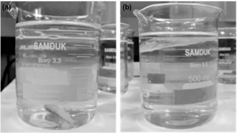
Measurements of density and sound speed contrasts The density contrast (g) is defined as the ratio of the density of the animals to that of the surrounding water (Chu and Wiebe 2005). For this measurement, we applied the density-bottle method in which fish mass density is determined by evaluating the buoyancy of each sample using a series of 500 mL beakers. These beakers contained water-glycerol solution of different density, ranging from 1.026 to 1.080 g/cm3 steps (Fig. 1). We defined the value of the bottle in which the fish were neutrally buoyant as fish mass density. If the fish was not neutral in any solution, the average between the last sinking bottle and the first floating bottle was taken. The density contrast of fish body g was obtained by dividing ρ by the density of seawater (ρsw= 1.025 g/cm³). The density of each bottle was confirmed using a glass aerometer and the solution in each bottle was kept at 25oC. Subsamples of 11 juvenile cod (58 ~ 79 mm) were used in the density measurements via density bottle method.
TS=20log Lfish
Fig. 1. Density measurement of juvenile cod by density bottle method. (a) shows fish density is greater than the density of solution, (b) is inverse case
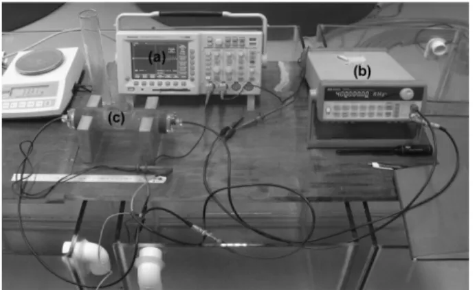
The sound speed contrast (h) is defined as the ratio of the sound speed in animals to those in the surrounding water (Chu and Wiebe 2005). The sound speed through the fish body was estimated by the time of flight method (Foote 1990). An acrylic ‘T-tube’ (inside diameter = 60 mm and inside length = 180 mm) was used for the measurement.
A continuous, sinusoidal-wave pulse of 400 kHz, 10µs was radiated from one side of the tube to the other by a function generator (HP 33120A, Hewlett Packard, USA), and the time it took the pulse to pass through the tube which containing seawater and fish was measured with a digital oscilloscope (TDS3054, Tektronix, Japan). The setting for the sound speed measurement is shown in Fig. 2.
In the time of flight method, an empirical equation issued to relate passing time through the mixture to the proportion of the volume filled by fishes V as
(2) where Tsw and Tfish are the “passing time” of sound through the sea water and though the fish body, respectively. The sound speed h is given by
(3)
Where Csw and Cfish are the speed of sound through seawater and fish body, respectively. As Csw is known from Tsw and the measurement distance (180 mm), can be deduced. The fish proportion V in previous equation was estimated by submerging a fish specimen in a graduated cylinder before the measurement. The T-tube was placed in a temperature-controlled tank and measure the change of pulse waves for sea water only as well as a mixture of sea water and fish specimen could be measured. the
measurement was carried out from 11oC to 19oC by 2oC steps.
Fig. 3 shows an example of the pulse wave data recorded by oscilloscope in the sound speed measurement.
It shows the pulse wave obtained from tube filled by seawater only and the other one filled with fishes. The passing time of the sound through the tube determined when the pulse wave began significantly changing the pattern. The phase differences were determined by the zero-cross method.
Estimation of target strength
A total 12 fish samples (Fig. 4) with their total length ranged from 52 to 105 mm were used in TS calculation from juvenile Pacific cod (Table 1). All fish were obtained from Gyeongsangnam-do Fisheries Resources Institute, Gyeongsangnam-do, South Korea. The samples were taken out of water were frozen immediately using dry ice Ttotal=(1 V– )Tsw+VTfish
h Tsw Tfish --- Cfish
Csw ---
= =
Fig. 2. Set of instrumentation for sound speed measure- ment. (a) oscilloscope, (b) function generator, (c) T-
tube Fig. 3. Example of the pulse wave data represents the
passing time of sound through the tube (a) filled by seawater (Tsw) and (b) filled by seawater and fishes (Tfish)
Fig. 4. Pacific cod (Gadus macrocephalus) used in this study
and added alcohol, and than x-ray photo of the shape, body and swim bladder of fish were taken. Examples of x- ray images of the juvenile Pacific cod are shown in Fig. 5.
Lateral and ventral images of the fish body and swim bladder were traced and then digitized at 1 mm intervals relative to the fish axis, fins and tail were not included in the trace. This digitized data was used to calculate the TS from the tilt angle and frequency using an acoustic scattering model.
3. Results
Density and sound speed contrast
The result showed that the value of body mass density
(ρ) ranged from 1.065 to 1.067 and its mean value was 1.066 (S.D. = 0.001). It is equivalent to density contrast (g) of 1.039~1.041 and 1.040, respectively. The distribution of fish samples, body mass density (ρ) and density contrast are shown in Table 2.
Due to the sound speed changes associated with temperature, we considered the range between 11o and 19oC for each 2oC step where the habitat temperature of cod is found. The sound speed of fish was higher than seawater within temperature range examined. The sound speed contrasts ranged from 1.003 to 1.029 with a mean of 1.014 (S.D. = 0.01). The sound speed through seawater, the sound speed through the fish and the sound speed contrast within each given temperature are listed in Table 3.
The number of fish used in the experiment were 20 individuals and the proportion of the volume V filled by fish was 0.13. The volume V denotes the ratio of the Table 1. Total length (TL) and body length (BL) of juvenile
cod samples
Sample No. TL (mm) BL (mm)
1 52 49
2 98 91
3 105 98
4 55 51
5 79 72
6 70 66
7 71 67
8 68 63
9 42 40
10 75 71
11 55 51
12 65 61
Mean 69.6 65.0
Fig. 5. Example of x-ray images to measure swim bladder and fish body from (a) lateral and (b) ventral view for using in the KRM model
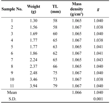
Table 2. Density contrast (g =ρfish/ρsw) of juvenile cod measured by density bottle method
Sample No. Weight (g)
TL (mm)
Mass density (g/cm³)
g
1 1.30 58 1.065 1.040
2 1.56 58 1.067 1.038
3 1.69 60 1.065 1.040
4 1.77 65 1.067 1.038
5 1.77 63 1.065 1.041
6 1.86 62 1.067 1.041
7 2.24 65 1.065 1.043
8 2.37 66 1.065 1.040
9 2.48 75 1.067 1.040
10 3.46 73 1.067 1.038
11 3.94 79 1.067 1.040
Mean 1.066 1.040
S.D. 0.001
Table 3. Sound speed contrast (h = Cfish/Csw) of juvenile cod measured by time of flight method
Temperature
(oC) Csw (m/s) Cfish (m/s) h
11 1491 1516 1.016
13 1498 1509 1.007
15 1504 1548 1.029
17 1511 1515 1.003
19 1516 1536 1.013
Mean 1.014
S.D. 0.01
volume occupied by fishes to the volume of seawater in the tube.
According to the references (Chu et al. 2003) in most
fish species, g ranges from 0.98 to 1.07 and h from 1.01 to 1.05, thus our results showed similar matching values.
Furusawa (1988) analyzed published data and determined that the most common values of g and h are 1.04 and 1.02, respectively, and hence these values are used in many models studies (Sawada et al. 1999).
TS estimation by KRM model
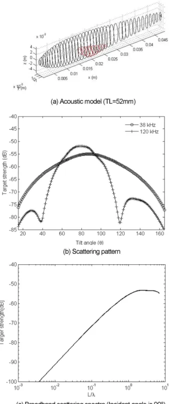
Typical examples of acoustic scattering characteristics for juvenile cod obtained by KRM model are shown in Fig. 6. TS pattern as function of tilt angle ranged from
−75o to 75o, from head-down to head-up, respectively at 38 and 120 kHz. The tilt angle is defined as the angle between the fish axis and the horizontal plane (Foote 1985). The average values of g and h were applied in the model calculations, 1.040 and 1.014, respectively.
In general, maximum target strength (TSmax) obtained at tilt angles between −5o to −1o (varied from −60.14 dB to
−45.37 dB) at 38 kHz and −14o to 1o (varied from −55.43 to
−42.33 dB) at 120 kHz with mean values about −3o and
−6o respectively. It means TSmax was detected when the fish was in head-down or near-horizontal position in both frequencies.
In this study, TS values for juvenile cod were estimated at two frequencies (38 and 120 kHz), which are commonly used in the acoustic surveys. The average target strength for tilt angle θ was estimated over the normal tilt angle distribution of the fish with probability density function (mean =−5o and standard deviation = 15o) (Foote 1980).
Moreover the ranges of TSmax and <TS> equations of the regression lines are shown in the Table 4.
The values of <TS> at two frequencies from total 12 fishes are plotted in Fig. 8 as function of total length in cm scale. The values at the frequency of 38 kHz and 120 kHz were varied between −60.42 to −46.62 and -57.83 to –49.12, respectively.
In fisheries acoustics, the standard form of the regression to set the slope is equal to 20 (Foote 1979). because back scattering is expected to be proportional to the cross- sectional area (L2) of a target (Love 1971; Foote 1979). A
Fig. 6. Typical acoustic scattering characteristics of juve- nile cod obtained by KRM model. (c) is plotted as function of total length (L) divided by wave- length (λ)
Table 4. Range of maximum TS (TSmax), average TS (<TS>) and equations of the regression lines f
(kHz) TS TS –
length equation R2 38 TSmax 37.9log(TL)− 82.3 0.87
<TS> 35.2log(TL)− 80.9 0.85 120 TSmax 33.7log(TL)− 76.0 0.87
<TS> 20.7log(TL)− 69.5 0.86
slope of 20 also allows populations or species to be compared using regression intercepts. As target strength- to-length regressions have been derived for more species, slopes with significant deviations from 20 have been found. Thus, by applying equation TS = 20log[TL(Total Length, cm)] + b, the relation between <TS> and length of juvenile cod were TS = 20log(TL)−68.8 (R2= 0.70) at 38 kHz and TS = 20log(TL)−69.4 (R2= 0.86) at 120 kHz (Fig. 7).
4. Discussion
Accuracy of estimated TS would be worse if density and sound speed contrasts were not accurate. Thus,
handling of model samples and making of them is important. The frozen samples used in the experiments were for modeling. Some authors have suggested that freezing and longer preservation time may cause significant changes in material conditions, such as water content and tissue composition, of marine organisms (McClathie et al.
1999; Benoit-Bird et al. 2008). However, the effect of freezing on tissue compositions should be minimum if the organisms are frozen quickly to lower temperatures (e.g.,
< −40oC) (Pruthi 1999). We used quick-freezing technique to freeze the samples, consequently the composition and condition of material did not change. Our samples were then moved and stored in fridge with temperature −40oC before used for measurements. This suggests no significant differences between live and frozen fish.
When Chu et al. (2003) investigated material properties of North Atlantic cod on the eggs and early-stage larvae where they obtained value of density contrasts for both stages, they found they were slightly less than unity (0.969 ~ 0.998), while value of sound speed-contrasts were greater than unity (1.017~1.024) and TS = 176.1log(TL)− 82 at 500 kHz. The result for density contrasts is different from our result, where g in our study was greater than unity (1.039~1.041). This difference represents the fact that density contrast changed quickly during the early growth stage. However, the sound speed contrast shows similar result that are slightly greater than unity.
Although this study only estimate the TS by theoretical model, there was still some evidence showing the good relationship between model and measured TS. Foote and Traynor (1988) indicated that TS of Walleye Pollock (Theragra chalcogramma) measured in situ at 38 kHz compared well to modeled results. However, modeled averages were consistently lower than measured results.
Abe et al. (2004) also conducted a study to compare the differences between measured TS and modeled TS of juvenile walleye Pollock (Theragra chalcogramma), they eventually obtained a good relationship results between them. Where the results show similar directivity of TS pattern however, maximum values of modeled TS are larger than those measured. Clay and Horne (1994) also found a good quality match between their models of adult Atlantic cod and measured results from dead, tethered cod reported at 38 kHz.
This is the first study report which provides the two important material properties and target strength of juvenile Pacific cod (Gadus macrocephalus). However there are only few other studies to be found for related species, especially Atlantic cod (Gadus morhua). Rose Fig. 7. The relationship between average TS and total
length (TL) of juvenile cod calculated by KRM model of fish at (a) 38 and (b) 120 kHz
and Porter (1996) reported that TS-length relationship of adult Atlantic cod were TS = 20log(TL)−66 at 38 kHz and TS = 20log(TL)−65 at 120 kHz measured by ex-situ.
Nielsen and Lundgren (1999) reported the ex-situ TS measurements of live juvenile cod (Gadus morhua L.) and their results shown the relationship of mean TS and log(TL) of juvenile cod at 120 kHz was 20log(TL)−68.0.
Also, in previous year, Ona 1994 performed in situ target strength measurements of juvenile cod in size 30 to 80 mm at 120 kHz obtained the TS - length relationship:
TS = 20log(TL)−70.
It is not easy to perform ex-situ TS measurement of juvenile cod using dual or split beam method such as collecting live samples, ensuring the seawater is a cold temperature for the live fish, and controlling tethered anesthetized fish to adjust tilt angles due to their size. In conclusion, our TS estimation would be a good guideline to verify the measurement values in the experiment.
Acknowledgement
The authors thank So-Gwang Lee, Ph D, Gyeongsangnam- do Fisheries Resources Research Institute, for providing live fish samples.
References
Abe K, Sadayasu K, Sawada K, Ishii K, Takao Y (2004) Precise target strength measurement and morphological observation of juvenile walleye pollock (Theragra chalcogramma). In: OCEANS '04. MTTS/IEEE, 9−12 Nov 2004
Benoit-Bird KJ, Gilly WF, Au WWL, Mate B (2008) Controlled and insitu target strength of the jumbo squid Dosidicus gigas and identification of potential acoustic scattering sources. J Acoust Soc Am 123(3):1318−1328 Chu D, Wiebe PH (2005) Measurements of sound speed and
density contrasts of zooplankton in Antarctic waters.
ICES J Mar Sci 62(4):818−831
Chu D, Wiebe PH, Copley NJ, Lawson LG, Puvanendran V (2003) Material properties of North Atlantic cod eggs and early-stages larvae and their influence on acoustic scattering. ICES J Mar Sci 60(3):508−515
Clay CS (1991) Low-resolution acoustic scattering models:
fluid-filled cylinders and fish with swim-bladders. J Acoust Soc Am 89(12):2168−2179
Clay CS (1992) Composite ray-mode approximations for backscattered sound from gas-filled cylinders and swim- bladders. J Acoust Soc Am 92(12):2173−2180
Clay CS, Horne JK (1994) Acoustic model of fish : the Atlantic cod (Gadus morhua). J Acoust Soc Am 96(3):
1661−1668
Foote KG (1979) Fish target-strength-to-length-regressions for application in fisheries research. In: Proceedings of the ultrasonic international 19, Graz, 15−17 May 1979, pp 327−333
Foote KG (1980) Averaging of fish target strength functions.
J Acoust Soc Am 67(10):504−515
Foote KG (1985) Rather-high-frequency sound scattering by swimbladdered fish. J Acoust Soc Am 78(4):688−700 Foote KG (1987) Fish target strengths for use in echo
integrator surveys. J Acoust Soc Am 82(5):981−987 Foote KG (1990) Speed of sound in euphausia superba. J
Acoust Soc Am 87(4):1405−1408
Foote KG, Traynor JJ (1988) Comparison of walleye pollock target strength estimates determined in situ measurements and calculations based on swim bladder form. J Acoust Soc Am 83(9):9−17
Furusawa M (1988) Prolate spheroidal models for predicting general trends of fish target strength. J Acoust Soc Jpn 9(1):13−24
Horne JK, Walline PD, Jech JM (2000) Comparing acoustic model predictions to in situ backscatter measurements of fish with dual-chambered swimbladders. J Fish Biol 57:1105−1121
Jech JM, Schael DM, Clay CS (1995) Application of three sound-scattering models to threadfin shad (Dorosoma petenense). J Acoust Soc Am 98(5):2262−2269
Kim MJ, An HS, Choi KH (2010) Genetic characteristics of Pacific cod populations in Korea based on microsatellite markers. Fish Sci 76(4):595−603
Love RH (1971) Measurements of fish target strength: a review. Fish Bull 69(4):703−715
MacLennan DN (1990) Acoustical measurement of fish abundance. J Acoust Soc Am 87(1):1−15
McClatchie S, Macaulay GJ, Coombs RF, Grimes P, Hart A (1990) Experiments on the target strength of the oily deepwater fish, orange roughy (Hoplostethus atlanticus).
Part I: experiments. J Acoust Soc Am 106(1):131−142 Nielsen JR, Lundgren B (1999) Hydroacoustic ex situ target
strength measurements on juvenile cod (Gadus morhua L.). ICES J Mar Sci 56(5):627−739
Ona E (1994) Detailed in situ target strength measurements of 0-group cod. ICES CM 1994/B:30, 9 p
Pruthi JS (1999) Quick freezing preservation of foods.
Allied Pub Ltd, New Delhi, 622 p
Rose GA, Porter DR (1996) Target-strength studies on Atlantic cod (Gadus morhua) in Newfoundland waters.
ICES J Mar Sci 53(2):259−265
Sawada K, Ye Z, Kieser R, Furusawa M (1999) Target strength measurements and modeling of walley pollock and Pacific hake. Fish Sci 65(2):193−205
Simmonds J, MacLennan D (2005) Fisheries acoustics.
Blackwell Publishing, Oxford, 456 p
Stanton TK (1989) Sound scattering by cylinders of finite
length III. Deformed cylinders. J Acoust Soc Am 86(3):
691−705
Received Jun. 8, 2015 Revised Oct. 21, 2015 Accepted Oct. 25, 2015