DOI http://dx.doi.org/10.11004/kosacs.2015.6.3.077
부피와 길이가 같은 변단면 기둥의 좌굴하중
이홍규1 ‧ 유종호1 ‧ 이승원1 ‧ 김선희2 ‧ 원용석3 ‧ 윤순종4
홍익대학교 토목공학과 석사과정1, 홍익대학교 토목공학과 박사수료2,
홍익대학교 토목공학과 박사과정3, 홍익대학교 토목공학과 교수4
Buckling Load of Columns with Same Volume and Length but Variable Cross-section along the Length
Lee, Hong-Kyu1⋅ Yoo, Jong-Ho1⋅ Lee, Seung-Won1⋅ Kim, Sun-Hee2
⋅ Won, Yong-Suk3⋅ Yoon, Soon-Jong4
1Graduate Reseach Assistant, Department of Civil Engineering, Hongik University, Seoul, Korea
2PhD. Candidate, Department of Civil Engineering, Hongik University, Seoul, Korea
3PhD. Student, Department of Civil Engineering, Hongik University, Seoul, Korea
4Professor, Department of Civil Engineering, Hongik University, Seoul, Korea
Abstract: In this paper, we present the result of investigations pertaining to the elastic buckling of simply supported columns with various cross-sectional dimensions but the same length and volume. In the investigations the accuracy of the analysis methods is studied and it was found that the result obtained by the successive approximations technique is the most accurate. In addition, the elastic buckling loads of columns with variable cross-section dimensions are obtained by the theoretical and numerical methods. From the results, it was found that the buckling loads obtained by the numerical methods are close to the buckling loads obtained by the successive approximations technique for the practical standpoints. Moreover, the buckling load of column with convexity in its middle is the highest while the buckling load of the tapered column is the lowest as expected.
Key Words: column with variable cross-section, buckling load, successive approximations technique, the finite element method
주요어: 변단면 기둥, 좌굴하중, 연속근사법, 유한요소법 Corresponding author: Yoon, Soon-Jong
Department of Civil Engineering, Hongik University, 72-1 Sangsu-dong, Mapo-gu, Seoul 121-791, Korea.
Tel: +82-2-320-1479, Fax: +82-2-3141-0774, E-mail: [email protected]
Received August 31, 2015 / Revised September 17, 2015 / Accepted September 19, 2015
1. INTRODUCTION
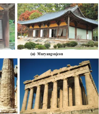
Columns with variable cross-section have been used in the architectural buildings around the world. Some illustrations of such columns are shown in Figs. 1 and 2. In addition, brief historical review of columns with entasis (a column with convexity in its middle) is given in the paper published by one of authors (Yoon et al., 2015).
In the design of column, the elastic buckling strength (or load) should be found. If the column is simply supported at its both ends and has uniform cross-section along the length (prismatic column) the elastic buckling load depends only on the elastic modulus E and the slenderness ratio l/r in which l is the length and r is the radius of gyration of the column (Timoshenko and Gere, 1961). However, if the column has variable cross-sectional area along the length of column there is no constant slenderness ratio.
Hence, the Euler buckling analysis is no longer
applicable.
In order to find the elastic buckling load of columns having various cross-sectional area along the length we may need other solution techniques such as the successive approximations technique, the finite element method, etc. If the column has the same length and volume but different cross-sectional area along its length it is interesting to find the buckling load in order to figure out which shape of columns results in the highest buckling load.
In this paper we present the result of investigations pertaining to the elastic buckling load of column with same length and volume but variable cross-sectional area along the length. In the investigations we adopted a column (for illustration) at the Muryangsujeon in Buseoksa-Temple, located in Youngju, Korea. The column is made of wood (Zelkova Serrata tree).
Detailed informations on the mechanical properties and dimension of the actual wooden column are discussed in the paper (Yoon et al., 2015). In the study, although wood is one of the typical natural composites with orthotropic nature of material, we assumed the material as isotropic but the effect of orthotropic material is taken into account.
(a) Muryangsujeon
(b) Parthenon
Fig. 1 Columns with Variable Cross-section
In this study, based on the actual dimension of column at the Muryangsujeon in Buseoksa-Temple, we modeled five columns having different cross-section dimension but approximately the same length and volume of each column.
In order to distinguish the difference between the columns visually, 1/25 scaled down model of columns are generated by the 3D printer as shown in Fig. 2.
Fig. 2 1/25 Scaled Down Column Models by the 3D Printer
2. MODELING OF COLUMNS
The mechanical properties (i.e., Ewood= 4.067GPa, wood = 0.490) and the dimension of actual circular wooden column are given in the paper (Yoon et al., 2015).
In this study, we fixed the length of circular cross-section columns to 3000mm. Each column is divided into 10 segments but 12 segments for H/3 convex column. Each segment is assumed to be prismatic (i.e., stepped configuration along the length) with circular cross-section. In order to make the columns have identical volume, AutoCAD (2010) program is used to change the diameter of segment in each column and the column named as Actual, Prismatic, H/2 Convex, H/3 Convex, and Tapered (refer to Fig. 2). Along the length of column the diameter and the moment of inertia for each segment are given in Tables 1 to 5, respectively.
Node No.
Diameter D (mm)
Moment of Inertia I (mm4)
0 367.500 1.00I0
1 425.438 1.80I0
2 453.188 2.31I0
3 472.063 2.72I0
4 485.875 3.06I0
5 492.250 3.22I0
6 494.188 3.27I0
7 494.625 3.28I0
8 488.813 3.13I0
9 480.438 2.92I0
10 460.625 2.47I0
Remark: I0=89.54×107mm4 Volume= 523.66×106mm3
Table 1. Diameter and Moment of Inertia of Actual Column
Node No.
Diameter D (mm)
Moment of Inertia I (mm4) 0
467.284 2.34×
1 2 3 4 5 6 7 8 9 10
Remark: I0=242.465×107mm4 Volume= 523.66×106mm3
Table 2. Diameter and Moment of Inertia of Prismatic Column
Node No.
Diameter D (mm)
Moment of Inertia I (mm4)
1 414.065 ×
2 452.940 ×
3 471.000 ×
4 483.345 ×
5 490.230 ×
6 490.230 ×
7 483.345 ×
8 471.000 ×
9 452.940 ×
10 414.065 ×
Remark: I0=144.29×107mm4 Volume= 523.66×106mm3
Table 3. Diameter and Moment of Inertia of H/2 Convex Column
Node No.
Diameter D (mm)
Moment of Inertia I (mm4)
0 430.00 1.00I0
1 440.00 1.10I0
2 448.60 1.18I0
3 459.61 1.31I0
4 470.00 1.43I0
5 482.00 1.58I0
6 493.00 1.73I0
7 503.00 1.87I0
8 510.00 1.98I0
9 490.00 1.69I0
10 470.00 1.43I0
11 450.00 1.20I0
12 430.00 1.00I0
Remark: I0=167.82×107mm4 Volume= 523.66×106mm3
Table 4. Diameter and Moment of Inertia of H/3 Convex Column
Node No.
Diameter D (mm)
Moment of Inertia I (mm4)
0 421.136 1.00I0
1 431.022 1.10I0
2 440.909 1.20I0
3 450.495 1.31I0
4 460.682 1.43I0
5 470.568 1.56I0
6 480.454 1.69I0
7 490.341 1.84I0
8 500.227 1.99I0
9 510.114 2.15I0
10 520.000 2.32I0
Remark: I0=154.40×107mm4 Volume= 523.66×106mm3
Table 5. Diameter and Moment of Inertia of Tapered Column
3. PREDICTION OF BUCKLING LOAD
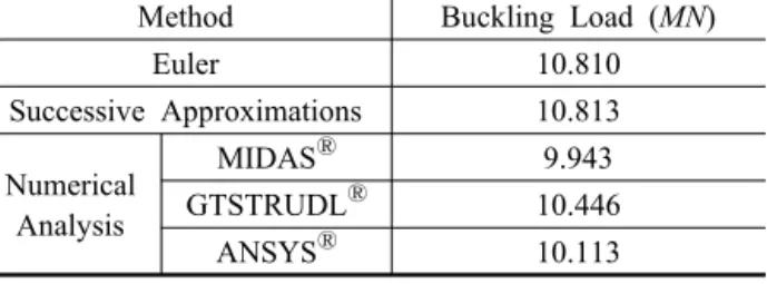
3.1 Successive Approximations Technique
If the diameter varies along the length of column Euler buckling analysis can not be applied. In this case we may use other approximate analysis techniques such as the successive approximations or the finite element techniques.
It was known that the successive approximations technique was developed by Schwartz and the mathematical verification on the accuracy of the
method was made by Trefftz.
It was also known that Engesser applied this method at first to the column buckling analysis (Timoshenko and Gere, 1961).
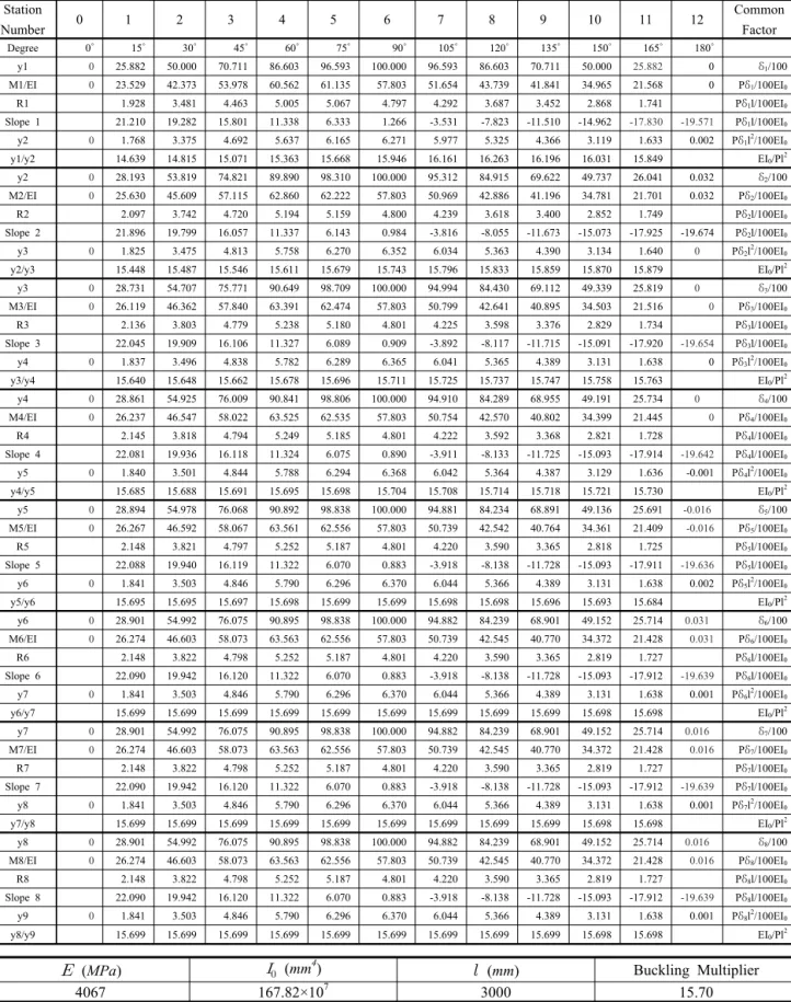
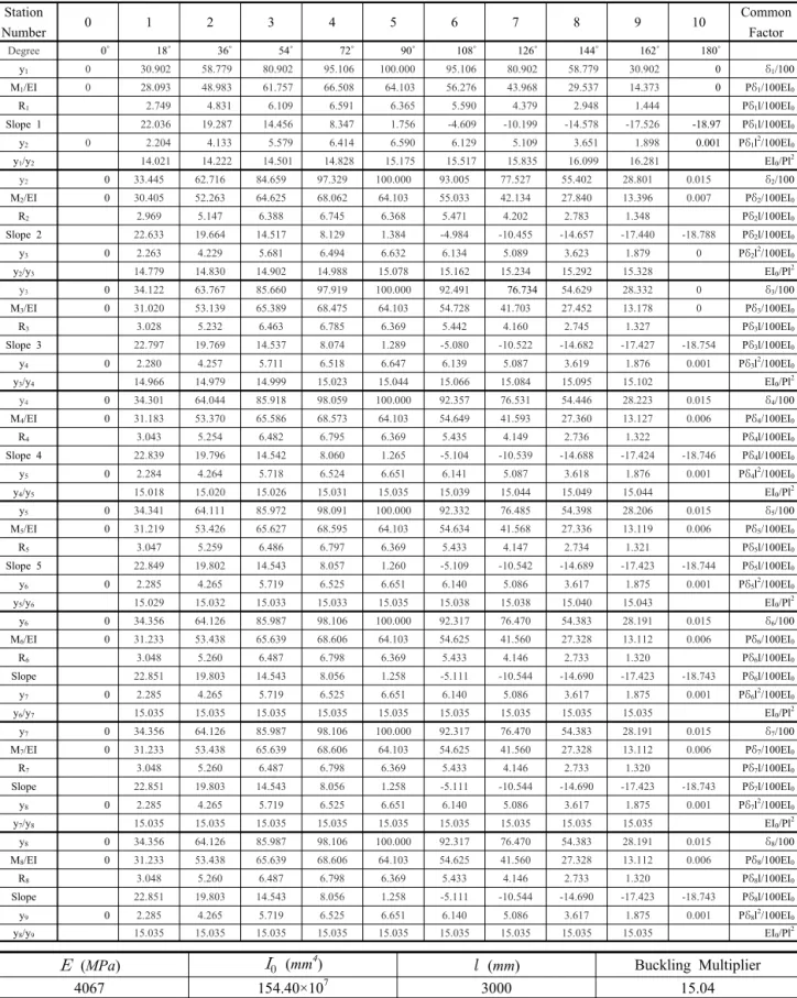
Detailed step by step calculation procedure is described by Lee (2015), Yoon (2015), and Timoshenko and Gere (1961), and complete results of calculation for five columns simply supported at both ends are given in Tables 8 to 12 attached in Appendix.
3.2 The Finite Element Analysis
Length of columns are fixed to 3000mm. Volume of each column is equal to 0.524m3 approximately.
Three commercially available finite element analysis programs, i.e., MIDASⓇ, GTSTRUDLⓇ, and ANSYSⓇ are used in the study.
The variable cross-section columns are modeled by AutoCADⓇ. The boundary condition at both ends of the column is modeled as simply supported and the concentrical compressive unit load is applied.
For illustration, one of the analysis results, the analysis model and buckled mode shape of the column obtained by each program, is shown in Figs. 3 to 5, respectively. Complete results of the finite element analysis performed by each program and obtained in each shape of columns are given in Tables 6 to 7 and also given by Lee (2015).
(a) Modeling (b) Buckled Mode Shape Fig. 3 Buckling Analysis by MIDAS®
(a) Modeling (b) Buckled Mode Shape Fig. 4 Buckling Analysis by ANSYS®
(a) Modeling (b) Buckled Mode Shape Fig. 5 Buckling Analysis by GTSTRUDL®
4. COMPARISON OF RESULTS
4.1 Accuracy of Results
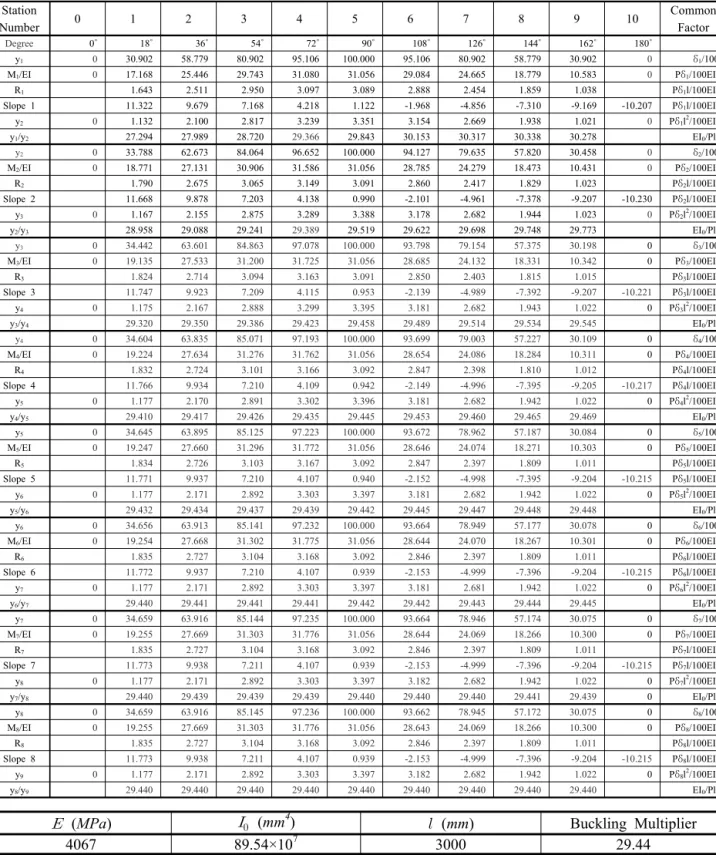
In order to figure out the accuracy of buckling load calculation, buckling loads of prismatic column obtained by the successive approximations and three finite element methods are compared with the Euler buckling load as given in Table 6. Euler buckling load is calculated by Eq. (1). In Eq. (1) E is the elastic modulus, I is the moment of inertia, and l is the length of column.
As can be seen in Table 6, the buckling load obtained by the successive approximations method differs +0.03% compared with the Euler buckling load.
Results obtained by the finite element analysis differ by –0.8% to +3.4%. It was found that the results obtained by either theoretical or numerical methods are accurate enough for the practical standpoints.
×
(1)
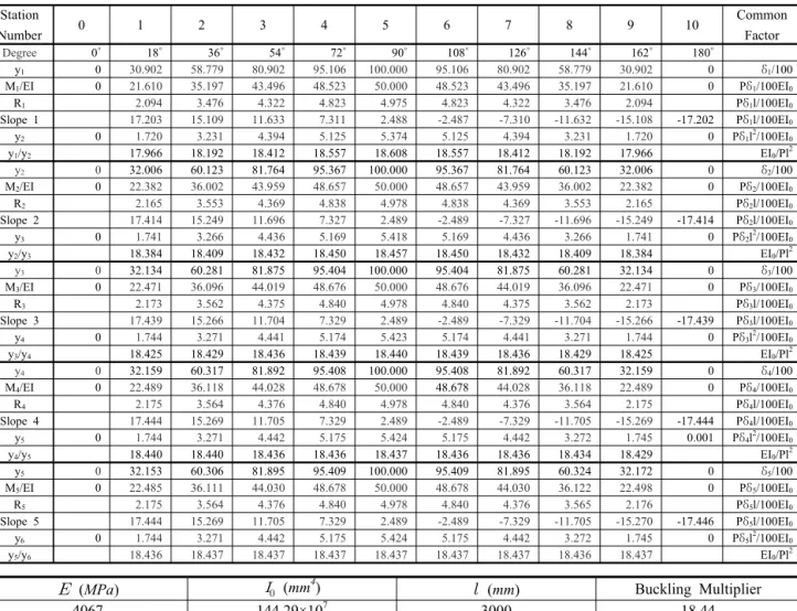
4.2 Comparison of Results
The buckling load of all columns, i.e., Actual, Prismatic, H/2 convex, H/3 convex, and Tapered are given in Table 7. From the study it was found that the result obtained by the MIDAS program yields the lowest buckling load compared with the successive
approximations result but the result is close enough for the practical purposes.
Method Buckling Load (MN)
Euler 10.810
Successive Approximations 10.813 Numerical
Analysis
MIDASⓇⓇⓇ 9.943
GTSTRUDLⓇⓇⓇ 10.446
ANSYSⓇⓇⓇ 10.113
Table 6. Comparison of Prismatic Column Results
Shape of Column
Buckling Load (MN)
MIDASⓇⓇⓇGTSTRUDLⓇⓇⓇ ANSYSⓇⓇⓇ Successive Approximations Prismatic 9.943 10.446 10.113 10.813
Actual 10.640 11.329 11.437 11.911 H/2 Convex 10.830 11.527 11.509 12.024 H/3 Convex 10.880 11.520 11.453 11.907 Tapered 9.576 10.063 10.160 10.490 Table 7. Comparison of Results
5. CONCLUSION
The buckling analysis on the columns with variable cross-section and simply supported at both ends is performed by the successive approximations technique and the finite element method. To confirm accuracy of methods, Euler buckling load of simply supported column is compared with the buckling loads obtained by other methods. The buckling load of prismatic column obtained by the successive approximations technique is almost the same but +0.03% higher. Also, the buckling loads obtained by the finite element methods are in the range between –0.8% to +3.4%
which are accurate enough for the practical standpoint.
As expected, the elastic buckling load for H/2 convex column is the highest while the buckling load for Tapered column is the lowest. If the buckling loads obtained by the successive approximations technique are compared with the buckling loads obtained by the numerical methods it was found that the results are in an acceptable range for the practical purposes.
ACKNOWLEDGMENT
This work was supported by 2014 Hongik University Research Fund. The financial support provided by the institution is appreciated.
References
ANSYSⓇ (2013), ANSYS Workbench 14.5.
AUTODESKⓇ (2010), AutoCAD 2010.
GTSTRUDLⓇ (2013), GTSTRUDL Ver. SE13.
Kiaei, M. (2011), “Variation in the Wood Physical and Mechanical Properties of Zelkova Carpinifolia Trees along Longitudinal Direction,” Middle-East Journal of Scientific Research, Vol. 9, No. 2, pp. 279-284.
Lee, S.-W. (2015), Buckling Analysis of Column with Variable Cross-section, Master Thesis, Department of Civil Engineering, Hongik University, Seoul, Korea (in Korean).
MIDASⓇ (2006), MIDAS Civil 2006.
Nam, J.-H., Son, K.-W., and Yoon, S.-J. (2004), “Flexural Analysis of Radiata Pine Plywood Plate for the Concrete Form by the Laminate Plate Theory,”
Mokchae Konghak, Vol. 32, No. 4, pp. 36-45.
Timoshenko, S. P. and Gere, J. M. (1961), Theory of Elastic Stability, Second Edition, McGraw-Hill, Inc., New York, USA.
Yoon, S.-J. (2015), Theory of Elastic Stability, Class Lecture Note, Department of Civil Engineering, Graduate School, Hongik University, Seoul, Korea.
Yoon, S.-J., Kim, H.-S., Yoo, H.-J., Han, M.-H., Kim, J.-K., and Ji, H.-I. (2015), “Buckling Strength of Wooden Column with Entasis at the Muryangsugeon in Buseoksa-Temple,” Journal of the Korean Society for Advanced Composite Structures, Vol. 6, No. 1, pp. 06-13.
Appendix
Station
Number 0 1 2 3 4 5 6 7 8 9 10 Common
Factor
Degree 0˚ 18˚ 36˚ 54˚ 72˚ 90˚ 108˚ 126˚ 144˚ 162˚ 180˚
y1 0 30.902 58.779 80.902 95.106 100.000 95.106 80.902 58.779 30.902 0 δ1/100
M1/EI 0 17.168 25.446 29.743 31.080 31.056 29.084 24.665 18.779 10.583 0 Pδ1/100EI0
R1 1.643 2.511 2.950 3.097 3.089 2.888 2.454 1.859 1.038 Pδ1l/100EI0
Slope 1 11.322 9.679 7.168 4.218 1.122 -1.968 -4.856 -7.310 -9.169 -10.207 Pδ1l/100EI0
y2 0 1.132 2.100 2.817 3.239 3.351 3.154 2.669 1.938 1.021 0 Pδ1l2/100EI0
y1/y2 27.294 27.989 28.720 29.366 29.843 30.153 30.317 30.338 30.278 EI0/Pl2
y2 0 33.788 62.673 84.064 96.652 100.000 94.127 79.635 57.820 30.458 0 δ2/100
M2/EI 0 18.771 27.131 30.906 31.586 31.056 28.785 24.279 18.473 10.431 0 Pδ2/100EI0
R2 1.790 2.675 3.065 3.149 3.091 2.860 2.417 1.829 1.023 Pδ2l/100EI0
Slope 2 11.668 9.878 7.203 4.138 0.990 -2.101 -4.961 -7.378 -9.207 -10.230 Pδ2l/100EI0
y3 0 1.167 2.155 2.875 3.289 3.388 3.178 2.682 1.944 1.023 0 Pδ2l2/100EI0
y2/y3 28.958 29.088 29.241 29.389 29.519 29.622 29.698 29.748 29.773 EI0/Pl2
y3 0 34.442 63.601 84.863 97.078 100.000 93.798 79.154 57.375 30.198 0 δ3/100
M3/EI 0 19.135 27.533 31.200 31.725 31.056 28.685 24.132 18.331 10.342 0 Pδ3/100EI0
R3 1.824 2.714 3.094 3.163 3.091 2.850 2.403 1.815 1.015 Pδ3l/100EI0
Slope 3 11.747 9.923 7.209 4.115 0.953 -2.139 -4.989 -7.392 -9.207 -10.221 Pδ3l/100EI0
y4 0 1.175 2.167 2.888 3.299 3.395 3.181 2.682 1.943 1.022 0 Pδ3l2/100EI0
y3/y4 29.320 29.350 29.386 29.423 29.458 29.489 29.514 29.534 29.545 EI0/Pl2
y4 0 34.604 63.835 85.071 97.193 100.000 93.699 79.003 57.227 30.109 0 δ4/100
M4/EI 0 19.224 27.634 31.276 31.762 31.056 28.654 24.086 18.284 10.311 0 Pδ4/100EI0
R4 1.832 2.724 3.101 3.166 3.092 2.847 2.398 1.810 1.012 Pδ4l/100EI0
Slope 4 11.766 9.934 7.210 4.109 0.942 -2.149 -4.996 -7.395 -9.205 -10.217 Pδ4l/100EI0
y5 0 1.177 2.170 2.891 3.302 3.396 3.181 2.682 1.942 1.022 0 Pδ4l2/100EI0
y4/y5 29.410 29.417 29.426 29.435 29.445 29.453 29.460 29.465 29.469 EI0/Pl2
y5 0 34.645 63.895 85.125 97.223 100.000 93.672 78.962 57.187 30.084 0 δ5/100
M5/EI 0 19.247 27.660 31.296 31.772 31.056 28.646 24.074 18.271 10.303 0 Pδ5/100EI0
R5 1.834 2.726 3.103 3.167 3.092 2.847 2.397 1.809 1.011 Pδ5l/100EI0
Slope 5 11.771 9.937 7.210 4.107 0.940 -2.152 -4.998 -7.395 -9.204 -10.215 Pδ5l/100EI0
y6 0 1.177 2.171 2.892 3.303 3.397 3.181 2.682 1.942 1.022 0 Pδ5l2/100EI0
y5/y6 29.432 29.434 29.437 29.439 29.442 29.445 29.447 29.448 29.448 EI0/Pl2
y6 0 34.656 63.913 85.141 97.232 100.000 93.664 78.949 57.177 30.078 0 δ6/100
M6/EI 0 19.254 27.668 31.302 31.775 31.056 28.644 24.070 18.267 10.301 0 Pδ6/100EI0
R6 1.835 2.727 3.104 3.168 3.092 2.846 2.397 1.809 1.011 Pδ6l/100EI0
Slope 6 11.772 9.937 7.210 4.107 0.939 -2.153 -4.999 -7.396 -9.204 -10.215 Pδ6l/100EI0
y7 0 1.177 2.171 2.892 3.303 3.397 3.181 2.681 1.942 1.022 0 Pδ6l2/100EI0
y6/y7 29.440 29.441 29.441 29.441 29.442 29.442 29.443 29.444 29.445 EI0/Pl2
y7 0 34.659 63.916 85.144 97.235 100.000 93.664 78.946 57.174 30.075 0 δ7/100
M7/EI 0 19.255 27.669 31.303 31.776 31.056 28.644 24.069 18.266 10.300 0 Pδ7/100EI0
R7 1.835 2.727 3.104 3.168 3.092 2.846 2.397 1.809 1.011 Pδ7l/100EI0
Slope 7 11.773 9.938 7.211 4.107 0.939 -2.153 -4.999 -7.396 -9.204 -10.215 Pδ7l/100EI0
y8 0 1.177 2.171 2.892 3.303 3.397 3.182 2.682 1.942 1.022 0 Pδ7l2/100EI0
y7/y8 29.440 29.439 29.439 29.439 29.440 29.440 29.440 29.441 29.439 0 EI0/Pl2
y8 0 34.659 63.916 85.145 97.236 100.000 93.662 78.945 57.172 30.075 0 δ8/100
M8/EI 0 19.255 27.669 31.303 31.776 31.056 28.643 24.069 18.266 10.300 0 Pδ8/100EI0
R8 1.835 2.727 3.104 3.168 3.092 2.846 2.397 1.809 1.011 Pδ8l/100EI0
Slope 8 11.773 9.938 7.211 4.107 0.939 -2.153 -4.999 -7.396 -9.204 -10.215 Pδ8l/100EI0
y9 0 1.177 2.171 2.892 3.303 3.397 3.182 2.682 1.942 1.022 0 Pδ8l2/100EI0
y8/y9 29.440 29.440 29.440 29.440 29.440 29.440 29.440 29.440 29.440 EI0/Pl2
Table 8. Successive Approximations (Actual Column)
(MPa) (mm4) (mm) Buckling Multiplier
4067 89.54×10⁷ 3000 29.44
×
×
Station
Number 0 1 2 3 4 5 6 7 8 9 10 Common
Factor
Degree 0˚ 18˚ 36˚ 54˚ 72˚ 90˚ 108˚ 126˚ 144˚ 162˚ 180˚
y1 0 30.902 58.779 80.902 95.106 100.000 95.106 80.902 58.779 30.902 0 δ1/100
M1/EI 0 30.902 58.779 80.902 95.106 100.000 95.106 80.902 58.779 30.902 0 Pδ1/100EI0
R1 3.065 5.830 8.024 9.433 9.918 9.433 8.024 5.830 3.065 Pδ1l/100EI0
Slope 1 31.311 28.246 22.416 14.392 4.959 -4.959 -14.392 -22.416 -28.246 -31.311 Pδ1l/100EI0
y2 0 3.131 5.956 8.198 9.637 10.133 9.637 8.198 5.956 3.131 0 Pδ1l2/100EI0
y1/y2 9.870 9.869 9.869 9.869 9.869 9.869 9.869 9.869 9.870 EI0/Pl2
y2 0 30.899 58.778 80.904 95.105 100.000 95.105 80.904 58.778 30.899 0 δ2/100
M2/EI 0 30.899 58.778 80.904 95.105 100.000 95.105 80.904 58.778 30.899 0 Pδ2/100EI0
R2 3.065 5.830 8.024 9.433 9.918 9.433 8.024 5.830 3.065 Pδ2l/100EI0
Slope 2 31.311 28.246 22.416 14.392 4.959 -4.959 -14.392 -22.416 -28.246 -31.311 Pδ2l/100EI0
y3 0 3.131 5.956 8.198 9.637 10.133 9.637 8.198 5.956 3.131 0 Pδ2l2/100EI0
y2/y3 9.869 9.869 9.869 9.869 9.869 9.869 9.869 9.869 9.869 EI0/Pl2
Table 9. Successive Approximations (Prismatic Column)
(MPa) (mm4) (mm) Buckling Multiplier
4067 242.465×10⁷ 3000.000 9.869
P r
×
×
Station
Number 0 1 2 3 4 5 6 7 8 9 10 Common
Factor
Degree 0˚ 18˚ 36˚ 54˚ 72˚ 90˚ 108˚ 126˚ 144˚ 162˚ 180˚
y1 0 30.902 58.779 80.902 95.106 100.000 95.106 80.902 58.779 30.902 0 δ1/100
M1/EI 0 21.610 35.197 43.496 48.523 50.000 48.523 43.496 35.197 21.610 0 Pδ1/100EI0
R1 2.094 3.476 4.322 4.823 4.975 4.823 4.322 3.476 2.094 Pδ1l/100EI0
Slope 1 17.203 15.109 11.633 7.311 2.488 -2.487 -7.310 -11.632 -15.108 -17.202 Pδ1l/100EI0
y2 0 1.720 3.231 4.394 5.125 5.374 5.125 4.394 3.231 1.720 0 Pδ1l2/100EI0
y1/y2 17.966 18.192 18.412 18.557 18.608 18.557 18.412 18.192 17.966 EI0/Pl2
y2 0 32.006 60.123 81.764 95.367 100.000 95.367 81.764 60.123 32.006 0 δ2/100
M2/EI 0 22.382 36.002 43.959 48.657 50.000 48.657 43.959 36.002 22.382 0 Pδ2/100EI0
R2 2.165 3.553 4.369 4.838 4.978 4.838 4.369 3.553 2.165 Pδ2l/100EI0
Slope 2 17.414 15.249 11.696 7.327 2.489 -2.489 -7.327 -11.696 -15.249 -17.414 Pδ2l/100EI0
y3 0 1.741 3.266 4.436 5.169 5.418 5.169 4.436 3.266 1.741 0 Pδ2l2/100EI0
y2/y3 18.384 18.409 18.432 18.450 18.457 18.450 18.432 18.409 18.384 EI0/Pl2
y3 0 32.134 60.281 81.875 95.404 100.000 95.404 81.875 60.281 32.134 0 δ3/100
M3/EI 0 22.471 36.096 44.019 48.676 50.000 48.676 44.019 36.096 22.471 0 Pδ3/100EI0
R3 2.173 3.562 4.375 4.840 4.978 4.840 4.375 3.562 2.173 Pδ3l/100EI0
Slope 3 17.439 15.266 11.704 7.329 2.489 -2.489 -7.329 -11.704 -15.266 -17.439 Pδ3l/100EI0
y4 0 1.744 3.271 4.441 5.174 5.423 5.174 4.441 3.271 1.744 0 Pδ3l2/100EI0
y3/y4 18.425 18.429 18.436 18.439 18.440 18.439 18.436 18.429 18.425 EI0/Pl2
y4 0 32.159 60.317 81.892 95.408 100.000 95.408 81.892 60.317 32.159 0 δ4/100
M4/EI 0 22.489 36.118 44.028 48.678 50.000 48.678 44.028 36.118 22.489 0 Pδ4/100EI0
R4 2.175 3.564 4.376 4.840 4.978 4.840 4.376 3.564 2.175 Pδ4l/100EI0
Slope 4 17.444 15.269 11.705 7.329 2.489 -2.489 -7.329 -11.705 -15.269 -17.444 Pδ4l/100EI0
y5 0 1.744 3.271 4.442 5.175 5.424 5.175 4.442 3.272 1.745 0.001 Pδ4l2/100EI0
y4/y5 18.440 18.440 18.436 18.436 18.437 18.436 18.436 18.434 18.429 EI0/Pl2
y5 0 32.153 60.306 81.895 95.409 100.000 95.409 81.895 60.324 32.172 0 δ5/100
M5/EI 0 22.485 36.111 44.030 48.678 50.000 48.678 44.030 36.122 22.498 0 Pδ5/100EI0
R5 2.175 3.564 4.376 4.840 4.978 4.840 4.376 3.565 2.176 Pδ5l/100EI0
Slope 5 17.444 15.269 11.705 7.329 2.489 -2.489 -7.329 -11.705 -15.270 -17.446 Pδ5l/100EI0
y6 0 1.744 3.271 4.442 5.175 5.424 5.175 4.442 3.272 1.745 0 Pδ5l2/100EI0
y5/y6 18.436 18.437 18.437 18.437 18.437 18.437 18.437 18.436 18.437 EI0/Pl2
Table 10. Successive Approximations (H/2 Convex Column)
(MPa) (mm4) (mm) Buckling Multiplier
4067 144.29×10⁷ 3000 18.44
×
×
Station
Number 0 1 2 3 4 5 6 7 8 9 10 11 12 Common
Factor
Degree 0˚ 15˚ 30˚ 45˚ 60˚ 75˚ 90˚ 105˚ 120˚ 135˚ 150˚ 165˚ 180˚
y1 0 25.882 50.000 70.711 86.603 96.593 100.000 96.593 86.603 70.711 50.000 25.882 0 δ1/100 M1/EI 0 23.529 42.373 53.978 60.562 61.135 57.803 51.654 43.739 41.841 34.965 21.568 0 Pδ1/100EI0
R1 1.928 3.481 4.463 5.005 5.067 4.797 4.292 3.687 3.452 2.868 1.741 Pδ1l/100EI0
Slope 1 21.210 19.282 15.801 11.338 6.333 1.266 -3.531 -7.823 -11.510 -14.962 -17.830 -19.571 Pδ1l/100EI0
y2 0 1.768 3.375 4.692 5.637 6.165 6.271 5.977 5.325 4.366 3.119 1.633 0.002 Pδ1l2/100EI0
y1/y2 14.639 14.815 15.071 15.363 15.668 15.946 16.161 16.263 16.196 16.031 15.849 EI0/Pl2 y2 0 28.193 53.819 74.821 89.890 98.310 100.000 95.312 84.915 69.622 49.737 26.041 0.032 δ2/100 M2/EI 0 25.630 45.609 57.115 62.860 62.222 57.803 50.969 42.886 41.196 34.781 21.701 0.032 Pδ2/100EI0
R2 2.097 3.742 4.720 5.194 5.159 4.800 4.239 3.618 3.400 2.852 1.749 Pδ2l/100EI0
Slope 2 21.896 19.799 16.057 11.337 6.143 0.984 -3.816 -8.055 -11.673 -15.073 -17.925 -19.674 Pδ2l/100EI0
y3 0 1.825 3.475 4.813 5.758 6.270 6.352 6.034 5.363 4.390 3.134 1.640 0 Pδ2l2/100EI0
y2/y3 15.448 15.487 15.546 15.611 15.679 15.743 15.796 15.833 15.859 15.870 15.879 EI0/Pl2
y3 0 28.731 54.707 75.771 90.649 98.709 100.000 94.994 84.430 69.112 49.339 25.819 0 δ3/100
M3/EI 0 26.119 46.362 57.840 63.391 62.474 57.803 50.799 42.641 40.895 34.503 21.516 0 Pδ3/100EI0
R3 2.136 3.803 4.779 5.238 5.180 4.801 4.225 3.598 3.376 2.829 1.734 Pδ3l/100EI0
Slope 3 22.045 19.909 16.106 11.327 6.089 0.909 -3.892 -8.117 -11.715 -15.091 -17.920 -19.654 Pδ3l/100EI0
y4 0 1.837 3.496 4.838 5.782 6.289 6.365 6.041 5.365 4.389 3.131 1.638 0 Pδ3l2/100EI0
y3/y4 15.640 15.648 15.662 15.678 15.696 15.711 15.725 15.737 15.747 15.758 15.763 EI0/Pl2
y4 0 28.861 54.925 76.009 90.841 98.806 100.000 94.910 84.289 68.955 49.191 25.734 0 δ4/100
M4/EI 0 26.237 46.547 58.022 63.525 62.535 57.803 50.754 42.570 40.802 34.399 21.445 0 Pδ4/100EI0
R4 2.145 3.818 4.794 5.249 5.185 4.801 4.222 3.592 3.368 2.821 1.728 Pδ4l/100EI0
Slope 4 22.081 19.936 16.118 11.324 6.075 0.890 -3.911 -8.133 -11.725 -15.093 -17.914 -19.642 Pδ4l/100EI0
y5 0 1.840 3.501 4.844 5.788 6.294 6.368 6.042 5.364 4.387 3.129 1.636 -0.001 Pδ4l2/100EI0
y4/y5 15.685 15.688 15.691 15.695 15.698 15.704 15.708 15.714 15.718 15.721 15.730 EI0/Pl2 y5 0 28.894 54.978 76.068 90.892 98.838 100.000 94.881 84.234 68.891 49.136 25.691 -0.016 δ5/100 M5/EI 0 26.267 46.592 58.067 63.561 62.556 57.803 50.739 42.542 40.764 34.361 21.409 -0.016 Pδ5/100EI0
R5 2.148 3.821 4.797 5.252 5.187 4.801 4.220 3.590 3.365 2.818 1.725 Pδ5l/100EI0
Slope 5 22.088 19.940 16.119 11.322 6.070 0.883 -3.918 -8.138 -11.728 -15.093 -17.911 -19.636 Pδ5l/100EI0
y6 0 1.841 3.503 4.846 5.790 6.296 6.370 6.044 5.366 4.389 3.131 1.638 0.002 Pδ5l2/100EI0
y5/y6 15.695 15.695 15.697 15.698 15.699 15.699 15.698 15.698 15.696 15.693 15.684 EI0/Pl2 y6 0 28.901 54.992 76.075 90.895 98.838 100.000 94.882 84.239 68.901 49.152 25.714 0.031 δ6/100 M6/EI 0 26.274 46.603 58.073 63.563 62.556 57.803 50.739 42.545 40.770 34.372 21.428 0.031 Pδ6/100EI0
R6 2.148 3.822 4.798 5.252 5.187 4.801 4.220 3.590 3.365 2.819 1.727 Pδ6l/100EI0
Slope 6 22.090 19.942 16.120 11.322 6.070 0.883 -3.918 -8.138 -11.728 -15.093 -17.912 -19.639 Pδ6l/100EI0
y7 0 1.841 3.503 4.846 5.790 6.296 6.370 6.044 5.366 4.389 3.131 1.638 0.001 Pδ6l2/100EI0
y6/y7 15.699 15.699 15.699 15.699 15.699 15.699 15.699 15.699 15.699 15.698 15.698 EI0/Pl2 y7 0 28.901 54.992 76.075 90.895 98.838 100.000 94.882 84.239 68.901 49.152 25.714 0.016 δ7/100 M7/EI 0 26.274 46.603 58.073 63.563 62.556 57.803 50.739 42.545 40.770 34.372 21.428 0.016 Pδ7/100EI0
R7 2.148 3.822 4.798 5.252 5.187 4.801 4.220 3.590 3.365 2.819 1.727 Pδ7l/100EI0
Slope 7 22.090 19.942 16.120 11.322 6.070 0.883 -3.918 -8.138 -11.728 -15.093 -17.912 -19.639 Pδ7l/100EI0
y8 0 1.841 3.503 4.846 5.790 6.296 6.370 6.044 5.366 4.389 3.131 1.638 0.001 Pδ7l2/100EI0
y7/y8 15.699 15.699 15.699 15.699 15.699 15.699 15.699 15.699 15.699 15.698 15.698 EI0/Pl2 y8 0 28.901 54.992 76.075 90.895 98.838 100.000 94.882 84.239 68.901 49.152 25.714 0.016 δ8/100 M8/EI 0 26.274 46.603 58.073 63.563 62.556 57.803 50.739 42.545 40.770 34.372 21.428 0.016 Pδ8/100EI0
R8 2.148 3.822 4.798 5.252 5.187 4.801 4.220 3.590 3.365 2.819 1.727 Pδ8l/100EI0
Slope 8 22.090 19.942 16.120 11.322 6.070 0.883 -3.918 -8.138 -11.728 -15.093 -17.912 -19.639 Pδ8l/100EI0
y9 0 1.841 3.503 4.846 5.790 6.296 6.370 6.044 5.366 4.389 3.131 1.638 0.001 Pδ8l2/100EI0
y8/y9 15.699 15.699 15.699 15.699 15.699 15.699 15.699 15.699 15.699 15.698 15.698 EI0/Pl2
Table 11. Successive Approximations (H/3 Convex Column)
(MPa) (mm4) (mm) Buckling Multiplier
4067 167.82×10⁷ 3000 15.70
×
×