Multi-Criteria decision making based on fuzzy measure
Yan Sun 1* , Di Feng 2
1
International Business School Suzhou, XJTLU, Suzhou 215123, China
2
Dept. of Electrical and Electronic Engineering, Suzhou 215123, China
요 약 치명적인 사고를 막기 위해 드라이버 졸음 (DD)를 검출하는 다양한 최근 방법이 제안되고있다. 본 논문은 운전자의 눈에 폐쇄 속도를 모니터링 할 수 있는 기능을 AdaBoost 기반 물체 검출 알고리즘에 적용한 DD 탐지 시스 템 구현에서 하드웨어/소프트웨어 공동 설계 방법을 제안한다. 소프트웨어 구성 요소는 DD 검출 알고리즘 중에서 필요한 기능성을 완전하게 달성하기 위해 전체적인 제어 및 논리 연산을 구현한다. 반면, 본 연구에서는 DD 검출 알고리즘의 중요한 기능은 처리를 가속화하기 위해 맞춤형 하드웨어 구성 요소를 통해 가속된다. 하드웨어/소프트웨 어 아키텍처는 비디오 도터 보드와 알테라 DE2 보드에 구현되었습니다. 제안 된 구현의 성능을 평가하고 몇 가지 최근의 작품을 벤치마킹했다.
Abstract Decision procedure was done with the evaluation of multi-criterion analysis. Importance of each criterion was considered through heuristically method, specially it was based on the heuristic least mean square algorithm. To consider coalition evaluation, it was carried out by calculation of Shapley index and Interaction value. The model output is also analyzed with the help of those two indexes, and the procedure was also displayed with details. Finally, the differences between the model output and the desired results are evaluated thoroughly, several problems are raised at the end of the example which require for further studying.
Key Words : Decision making, heuristic least square, Shapley index, interaction index, fuzzy membership function
접수일 : 2013년 8월 10일 수정일 : 2013년 9월 22일 게재확정일 : 2013년 10월 8일
*교신저자 : Yan Sun([email protected])
1. Introduction
Decision making has been studied by numerous researches [1, 4 and references there in]. Obtained decision algorithm can be applied to engineering, industrial design, and economics through the decision of control value, scheduling, and when buy or sell, and how many, and so on. In order to get reasonable decision result, it is required to conduct the calculation based on optimization or rational approach. There are several ways of conducting optimization with least mean square algorithm [1].
With the first application of the concept of fuzzy
measure to the field of multi-criteria decision making
was done in 1974 by Sugeno [2], in which he described
the fuzzy measure as an efficient and validity method
of evaluation real problem. By considering the fuzzy
set, in which elements have flexible membership values
such as inbetween zero and one. It means that fuzzy
set can provide more general expression than
mathematical characteristic function including
individual opinion [4]. Actually, starting from Zadeh
fuzzy theory has provided solutions of control, image
processing, game theory, and pattern recognition and
other multiple research areas. By assigning the fuzzy
membership function, we could evaluate degree of
uncertainty and similarity through designing of fuzzy entropy and similarity measure [6-10]. With the help of fuzzy entropy and similarity, it was also provided solution of clustering, reliable data selection [9,10].
Because of these flexible characteristics, it constitutes the expert system with neural network. Specially, it provided very efficient supporting tool for human decision of strategies [3,4]. Decision theory has been studied as rationale basis, its related topics deal optimization with/without constraint, linear and nonlinear optimization. Including control strategies, multiple strategies can be composed as candidates of solution. In order to get solution, it should need to consider constraint, whether it is uni/multi-criteria, whether it satisfies coalition or not.
In this literature, decision under the condition of multi-criteria was considered, which means that we have to consider multiple constraint or condition to get proper decision. With an illustrative example, a complete system of making decision will be established to the reader. This example acts as the main clue of the report and the author will establish all relative values with detail process of calculation. The primary purpose of this paper lays on recording the process of the author studying others’ outcomes, which may help him or others to have a better understanding of the algorithm and the method.
An illustrative is firstly given with detail description, and then an algorithm invented by Michel Grabisch [3]
is cited to solve this problem by modeling real condition into numerical values. Also, global score is given with analyzing of the instructor. Finally, Shapley index and Interaction index are calculated to show the process of making decision and then the model outputs are calculated. However, several problems are coming with the output of the model, they are expected to be solved with further study.
2. Preliminaries
2.1 Heuristic Least Mean Squares (HLMS)
In order to minimize the distance between the given results and the calculated one, judging algorithm is proposed. Applying this principle, if the distance is too large then result cannot be reliable, and the model may need further modifications. HLMS is considered from the idea of Least Mean Squares (LMS) by Grabisch derived [3]. Because representation is difficult to calculate for a large number of criteria, and the standard optimization algorithms are not suitable to fuzzy measures. It also showed better performance than the algorithm raised by Mori and Murofushi [5].
HLMS uses the obtained data to do a series calculation and represent fuzzy measures in the finite case by using a lattice representation.
Consider the Fig. 1 as the lattice, in which four values of criteria are treated as a four-dimension matrix (e.g. [
,
,
,
]), the global score given by the instructor is also a necessary input as well.
Algorithm constitutes three steps as follows.
・ Step 1: The lattice representation is initialized at the equilibrium state. The equilibrium state is that the first level in the above representation is zero, and every level is equal to the value of previous level add to 0.25, and finally the last level have the value of 1.
Fig. 1. Lattice structure of four criteria
・ Step 2: Convert the value in Table 1 and global
score into the form of datum (
,
,
,
, ) and
compute the error of the model:
=
( - (1)
Then we can modify the point in the lattice by the following equation:
≠ =
-
(
-
) (2)
n the above equation, represent the location of the point.
is 1 in this example and is 4. Then we have to verify the monotonicity, if verification is done, the value is changed and if the monotonicity is violated then the value will not be modified.
・ Step 3: For the node that unmodified in the previous step, first verify them by using the upper and lower neighbors, and then modify them using method just introduced. For the case that the upper and lower neighbors that do not satisfy the monotonicity there is another method applied. Before introducing the method, several factors should be introduced. =/(-)
, , = /(-) and are denote minimum distance between and its upper neighbors, and minimum distance between and its lower neighbors, respectively.
For +
- 2() > 0,
=
+
(3) Otherwise,
=
+
(4)
2.2 Important indexes 2.2.1 Shapley index
Shapley index is considered as an average value of one item that contributed to the whole system, it is an
important index that helps decision maker to understand the importance of every criterion. It is calculated by the following equation:
=
⊂ \
∪ (5)
is a collection of all possible combinations of criterion except criterion .
2.2.2 Interaction index
Interaction index is used to display the relationship between different elements, it also has the equation to compute numerical value.
=
⊂ \
[( ∪{,})-( ∪{})-( ∪{})+( )] (6)
Again, is a collection of all possible combination of elements except and and | | is the number of members of set . The effect of one criterion is different from the other one. In the Multi-criteria case, the algorithm firstly offers the data and then the importance of every criterion and their relationship can be established in a clear form by using Shapley index and Interaction index. A coalition is a treaty among groups or individuals (between two criteria in this case), during which they have joint part [4]. It has significant effects on calculating the interaction index, which is most informative. With the instruction of the interaction index, the importance of the coalition is obviously and can help the reader to judge and evaluate the behavior of the instructor.
3. Decision Algorithms
3.1 Descrption of the example
In this example, we consider the problem of the
selection of electrical products. Different kinds of
products are evaluated based on the following four criteria.
・ Cost: Price is an important criterion, and it will be converted into numerical score. Under 600 CNY is best choice and over 1000 is unacceptable.
・ Life span: The time period that the product can work properly is also taken as one criterion. Less than 2 years is totally unacceptable and over 10 years is the best choice.
・ Popularity: This criterion shows how many people recommend these products which can be treated as a kind of guarantee. The score going from A(Recommend) To E(Not recommend), it may not be accurate.
・ Stability: Qualitative score is given by the instructor, going from A(perfect match) to E(Unstable)
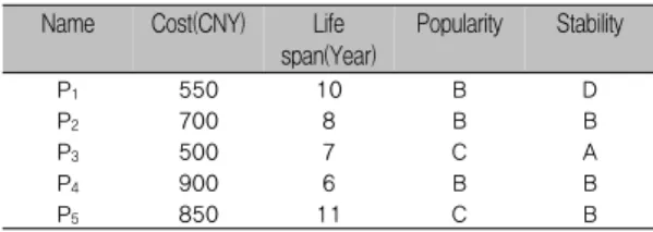
Five products are considered, name from P1 to P5.
The following table displays their performance on every criterion.
Name Cost(CNY) Life span(Year)
Popularity Stability
P
1550 10 B D
P
2700 8 B B
P
3500 7 C A
P
4900 6 B B
P
5850 11 C B
Table 1. Product evaluation over 4 criteria
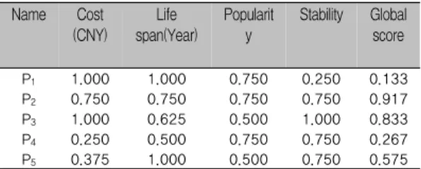
3.2 Conversion principle and evaluation based on utility function
By applying the utility functions, the numerical score based on different criteria can be given in Table 2.
Global score is indicated by the instructors. And the following paragraph will give detail description about how to divide those five products into three groups. For the product
, it has a cheap price and long life span and there are a large number of people recommending this product, however, the degree of satisfaction to our system is only 0.25 which is unacceptable. Thus, it
belongs to the last class. Product
has an acceptable price and long enough life span, while many people also recommend this one. For the stability, it can fit our system, but there also exist the possibility that the system will break down which makes this product belongs to first class. The balance distribution of score make it is the best choice for the instructor. Product
costs least to the instructor, but it have a relative short life span. And there are few people recommending this one which indicated some unknown latent shortcomings. This one can fit the system very well, almost no possibility to trigger the failure, which also makes it belongs to the first class. But based on overall consideration, it has less validity and practicability than product
. Product
costs most in five products a relative short life span, but some customers also recommend this one due to its high stability. Based on the cost and life span it should be put into the last class but the high stability makes it better than P1. Product
just costs slightly less than
but it has the longest life span. For the popularity, there are several people ever used it which make the information may not be accurate but it has a relative high performance in stability. Considering four criteria, it will be label as average.
Then we can obtain the priority among five products, that is:
>
>
>
>
and
belong to the first class,
is in the
average level while
and
come from the third
class. Because the fuzzy measures regard 1 as the fully
satisfied and 0 as totally unacceptable, we can put
these five points on one line distribution and then the
global score can be obtained. Recall the method given
by Michel Grabisch [3], we can put the global score
interval for first class to be [1, 0.75], [0.75, 0.4] for the
average level and [0.4, 0] for the third class. Then the
Table 2 is generated based on descriptions and Table
1 to which is:
Name Cost
(CNY) Life span(Year)
Popularit y
Stability Global score
P
11.000 1.000 0.750 0.250 0.133 P
20.750 0.750 0.750 0.750 0.917 P
31.000 0.625 0.500 1.000 0.833 P
40.250 0.500 0.750 0.750 0.267 P
50.375 1.000 0.500 0.750 0.575
Table 2. Evaluation of 4 criteria via utility function andglobal score
3.3 Lattice representation
First we have to set ==0.05 and iteration to be 300. Iteration means the times that every point been modified or verified according to the HLMS. In this case, every point conducts a series of steps that just introduced for 300 times.
⊘= 0,
= 0.17,
= 0.175,
= 0,
= 0,
= 0.175,
= 0.175,
= 0.613,
= 0.175,
= 0.425,
= 0,
= 0.175,
= 0.788,
= 0.74,
= 0.425,
= 1
Shapley index
Recall the equation (5), if we set =, ={,,}
then has eight kinds of combination, we illustrate two of them as follows
= {},
[-]
= {,,},
[-]
The summation of above eight equations is 0.343535.
Applying this method and we can get the Shapley index for the other criteria which are displayed in the following table.
It is not hard to find out that stability is the most important criterion when conducting the decision and popularity has the least significance. For the cost and life span, they influence the decision made by the
instructor, however, it does not as important as stability. Then we can make the conclusion that cost and life span show their importance only under the condition that the degree satisfaction of stability is large enough (0.75 and larger, indicated by the instructor)
Interaction index
Recall equation (6), if we set = and = then =
{,}, there are following four kinds of possibility.
= {⊘};
[--+⊘]
= {};
[--+]
= {};
[--+]
= {,};
[--+]
The summation of above four parts is -0.182492 Applying this method and we can get the interaction index for the other criteria which are displayed in the Table 3.
Interaction index
Value Shapley index
Value
a, b -0.182492 Cost 0.343535 a, c 0.093900 Life
span
0.209463
b, c 0.027545 Popularity 0.064143 a, d 0.493931 Stability 0.382806 b, d 0.239819
c, d 0.090860
Table 3. Values of interaction index/ Value of Shapley index
From this table we can find that the interaction of
a and b is negative while others are positive. The
negative one indicates that criterion a and b can
compensate each other. And there are significant
positive interaction index between a, d, and b, d, which display the fact that stability is the most important criterion.
Model output
The Shapley index and interaction index influence the output of the model. There is an equation of Choquet integral for 2-additive measures, that is:
(
,...,
)=
∧
+
∨
+
≠
(7)
Equation can be divided into three parts, the following procedures use product
as an example to display the process of calculating. The values for criteria on
are 1, 1, 0.75 and 0.25. Recall the values in Table 3, the calculation can be processed without problem.
For the first two parts the result is
0.75×0.1+0.75×0.0275+0.25×0.5+0.25×0.24+0.25×0.09+1
×|-0.18| = 0.3
The last part has four conditions.
=1,
1×(0.343535-0.5×(0.182492+0.09390+0.5))=-0.0416262
=2,
1×(0.2-0.5×(0.182492+0.027545+0.24))=-0.015465
=3,
0.75×(0.064143-0.5×(0.1+0.027545+0.09))=-0.031507
=4,
0.25×(0.382860-0.5×(0.5+0.239819+0.09))=-0.007361
The summation of above three items is 0.383769, and by the same procedure we can obtain the other four model outputs. The relative data are established in the following table.
Product name
Model output Desire output
P
10.383769 0.133333
P
20.750002 0.916667
P
30.830721 0.833333
P
40.368300 0.266667
P
50.567847 0.575000
Table 4. Output of the lattice representation and desire value