A Novel Localization Algorithm using Received Signal Strength Difference

(1)

1. INTRODUCTION

The ability to accurately locate the position of a radio emitter is often of vital importance in civilian and military applications. There are various emitter geolocation techniques, each having specific advantages and disadvantages (Hata 1980). Recent interest in geolocation techniques based on measurements of received signal strength (RSS) has been motivated by the possibility of networking simple sensors using wireless communications technology to obtain useful geolocation performance capabilities. Practical advantages include the elimination of requirements for the complex array antennas associated with conventional angle of arrival techniques and the demanding time synchronization needed to implement time and frequency difference of arrival geolocation techniques. Consequently, RSS techniques can be attractive even if a relatively large number of sensors is needed to achieve the required accuracy.

The general concept of RSS geolocation is to estimate

A Novel Localization Algorithm using Received Signal Strength Difference

Deok Won Lim

^†

, Jae-Hee Seo, Sebum Chun, Moon Beom Heo

Satellite Navigation Team, Korea Aerospace Research Institute, Daejeon 305-806, Korea

ABSTRACT

In this paper, an efficient and robust localization algorithm using Receiver Signal Strength Difference (RSSD) for a non- cooperative RF emitter is given. The proposed algorithm firstly calculate the center point and radius of Apollonius’s circles and then estimate the intersection point of the circles based on Time of Arrival concept. And this paper also compares the performance of RSSD localization algorithms such as Non-linear Least Squares and Linearized Least Squares by Lines of Position (LOP) with the proposed algorithm. And some conclusions have been reached regarding the relative accuracy, robustness and computational cost of these algorithms.

Keywords: localization, received signal strength difference, non-cooperative RF emitter

an emitter location that is consistent with the power measurements obtained from sensors distributed in the area of interest. Given a propagation model that provides a statistical relationship between received signal power and the emitter to sensor separation along with a priori knowledge of the transmitted power, the distance between each receiver and the emitter can be estimated using properly calibrated measurements of the received signal power. This approach implies a cooperative emitter and the emitter is assumed to operate with a known effective radiated power and an omnidirectional radiation pattern.

The requirement for a cooperative emitter can be substantially avoided by the use of RSS difference (RSSD).

The basic concept is that the ratio of the signal powers (or their differences expressed in dB) observed at two spatially separated sensors is related to the ratios of the emitter to sensor distances. The solution of the emitter position using RSSD information from multiple pairs of sensors is a more complex problem than that of the analogous RSS geolocation problem with a priori knowledge of transmitted power.

A simple geometric interpretation for RSS difference based localization can be illustrated by considering a plane containing a single pair of receivers and an emitter.

If the path loss follows a simple inverse power law, the RSS difference (in decibels) between the two receivers can be Received July 10, 2017 Revised July 31, 2017 Accepted Aug 02, 2017

†

Corresponding Author E-mail: [email protected]

Tel: +82-42-870-3978 Fax: +82-42-860-2789

(2)

shown to define a circle which is to be Apollonius’s circle and the emitter must lie on it. With additional receivers, the position of the emitter can be solved by finding the common intersection of the circles corresponding to the different pairs of receivers.

This paper presents an efficient and robust least squares solution which utilizes the measured center points and radius of Apollonius’s circle. And this paper also compares the performance of several RSSD localization algorithm implementations for non-cooperative emitters. Simulated data are used to compare the localization accuracy of these algorithms. Some conclusions have been reached regarding the accuracy and computational cost of these algorithms.

2. GEOMETRIC INTERPRETATION OF RSSD

2.1 Empirical Path Loss Model

Empirical path loss models are useful for estimating the RSS as a function of parameters such as propagation distance, d, emitter’s antenna height, h

t

, receive antenna height, h

r

, and the carrier frequency of the emitted signal, f (Hata 1980, Xia 1996, Alam et al. 2010). Although these models differ in details, the dependence of the RSS on the emitter to receiver separation is generally expressed as a power law of the form:

r

A

t

P P

d

^γ

= , (1)

where P

t

is the transmitted signal power, A = A(h

t

, h

r

, f) is a positive constant that depends on h

t

, h

r

, f and r >2 is a positive constant, called the path loss exponent. Here d >0 must be sufficiently large to avoid near-field effects.

In logarithmic scale, Eq. (1) can be reformulated as

( )

( ) ( )

( )

10

10 10

10

10log

10log 10 log

10 log

r t

P

AP d

C d

γ γ

Ω =

= −

,

(2)

where C = C(h

t

, h

r

, f , P

t

) = 10log

10

(AP

t

). If h

r

, h

t

, f and P

t

are fixed, C will essentially be a constant for all receivers (Alam et al. 2010). This model is widely used in RSS based geolocation (Xia 1996, Weiss 2003, Alam et al. 2010).

2.2 A Geometric Interpretation of RSS Difference Based Geolocation

The possibility of geolocating a radio frequency emitter using RSS measurements obtained from simple sensors has

motivated much recent research (Cheung et al. 2003, Weiss 2003, Alam et al. 2010). For uncooperative emitters, a priori knowledge of the transmitted signal power is not available and it is necessary to obtain solutions in terms of the relative RSSs observed at different locations. This approach has a simple geometric interpretation.

Consider an RF emitter at T = (x, y) and two receivers at R

1

= (x

1

, y

1

) and R

2

= (x

2

, y

2

). Denote the distances from R

1

and R

2

to T by d

1

and d

2

, respectively, and the each distance can be represented as

( ) (

²

)

²

1 1 1

d = x x − + y y − , (3)

and

( ) (

²

)

²

2 2 2

d = x x − + y y − . (4)

Let the RSS (in dBm) R

1

and R

2

be denoted by Ω

1

and Ω

2

respectively and define Ω

₁₂

≡ Ω

1

- Ω

₂

. Then, according to Eq. (2),

12 10 2

10 log d d γ ^

1

^

Ω =     , (5)

where the constant but unknown parameter C cancels out.

Let

512 12

10

^γ

α ≡

^Ω

, (6)

Eq. (6) can then be rewritten as

( x x −

₂

) (

²

+ y y −

₂

)

²

= α

₁₂

^  ( x x −

₁

) (

²

+ y y −

₁

)

²

^  , (7) If α

12

≠ 1, Eq. (7) can be rewritten as

( )

2 2 2

2 12 1 2 12 1 12 12

12 12 12 2

1 1 1

x x y y d

x α y α α

α α α

 − −  +  − −  =

 −   −  −

    , (8)

which represents a circle with radius

( )

12

12 122 2

1

12

c

d

R α

= α

− and

center.

12 12

2 12 1 2 12 1

12 12

( , ) ,

1 1

c c

x x y y

x y α α

α α

 − − 

=   − −   . (9)

Since each pair of receivers generates a circle on which

the emitter lies, the problem of localizing the RF emitter

is reduced to that of finding the common intersection

of multiple circles in some optimal manner. The circles

associated with pairs of receivers are analogous to lines

of bearing in angle of arrival based geolocation. As an

illustration, the circles associated with the 10 possible pairs

of receivers out of a total of 5 receivers are plotted in Fig. 1

(Wang & Inkol 2011), where the circles intersect at a single

(3)

point at which the emitter is located.

3. GENERAL RSSD ALGORITHMS FOR A NON-COOPERATIVE EMITTER

This section describes several RSSD algorithms for the geolocation estimation of non-cooperative emitters. First, the Non-linear Least Squares (NLS) method is detailed.

3.1 Non-linear Least Squares

Using Eqs. (3) and (4) along with Eq. (5) (Cheung et al.

2003, Jackson et al. 2011),

( ) ( )

2 2

12 1 2 10 2 2

1 1

5 log x x y y

x x y y

γ ^ ⁻ ⁺ ⁻ ^

Ω = Ω − Ω =    − + −    . (10)

In general, if there are N sensors, and 1 ≤ k < l ≤ N

( ) ( )

2 2

10 2 2

5 log

^l ^l

kl k l

k k

x x y y

γ ^ ⁻ ⁺ ⁻ ^

Ω = Ω − Ω =    − + −   

. (11)

If the actual measured power difference between the receivers at R

k

= (x

k

, y

k

) and R

l

= (x

l

, y

l

) is _

P

kl

, the optimal NLS method finds the (x, y) that minimize the sum of the squares of the differences between the actual measured received signal strengths and the theoretical received signal strengths given by (Jackson et al. 2011),

which represents a circle with radius

 

12

12 122 2

1

12

c

d

R 

 

 and center.

12 12

2 12 1 2 12 1

12 12

( , ) ,

1 1

c c

x x y y

x y  

 

   

       . (9)

Since each pair of receivers generates a circle on which the emitter lies, the problem of localizing the RF emitter is reduced to that of finding the common intersection of multiple circles in some optimal manner. The circles associated with pairs of receivers are analogous to lines of bearing in angle of arrival based geolocation. As an illustration, the circles associated with the 10 possible pairs of receivers out of a total of 5 receivers are plotted in Fig. 1 (Wang & Inkol 2011), where the circles intersect at a single point at which the emitter is located.

3. GENERAL RSSD ALGORITHMS FOR A NON-COOPERATIVE EMITTER

This section describes several RSSD algorithms for the geolocation estimation of non- cooperative emitters. First, the Non-linear Least Squares (NLS) method is detailed.

3.1 Non-linear Least Squares

Using Eqs. (3) and (4) along with Eq. (5) (Cheung et al. 2003, Jackson et al. 2011),

   

2 2

12 1 2 10 2 2

1 1

5 log x x y y

x x y y

 ^ ^ ^ ^ ^

               . (10)

In general, if there are N sensors, and 1 k l N   

   

2 2

10 2 2

5 log

^l ^l

kl k l

k k

x x y y

 ^ ^ ^ ^ ^

       

    

  . (11) If the actual measured power difference between the receivers at R

_k

 ( , ) x y

_k _k

and ( , )

l l l

R  x y is P , the optimal NLS method finds the ( , )

_kl

x y that minimize the sum of the squares of the differences between the actual measured received signal strengths and the theoretical received signal strengths given by (Jackson et al. 2011),

   

2 2 2

10 2 2

( , )

kl

5 log

^l ^l

k l k k

x x y y

Q x y

x x y y





      

 

                 , (12) , (12) for all combinations of receiver pairs. The objective

function Q is non-linear and the only reliable method to find its minimum is to define a grid over which a search

is conducted with Q evaluated at each point on the grid.

Ultimately, the grid point that minimizes Q is selected as the position fix for the emitter. Since a search grid must be defined, there is a direct correlation between computation time and emitter geolocation accuracy.

3.2 Linear Least Squares by LOP

Some papers use a geometrical approach (Caffery 2000), which generates linear lines of position (LOP) by differencing pairs of circular LOPs and proceeds to solve the Mobile Station location using the least-squares algorithm (Juang et al. 2006). The linear LOP determined by two circles, centered at ( x

c12

, y

c12

) and ( x

c13

, y

c13

) with radiuses of R

12

and R

13

, respectively, is given by

12 12 13 13

13 12 13 12

2 2 2 2

12 13

( ) ( )

2

c c c c

R R x y x y

x x x y y y − − + + +

− + − = . (13)

For simplicity, setting N = 3 and expressing the set of linear LOPs in matrix form,

s MS s

A X = B , (14)

where

13 12 13 12

23 12 23 12

23 13 23 13

c c c c

s c c c c

c c c c

x x y y

A x x y y

x x y y

 − − 

 

=  − − 

 − − 

 

 

,

_MS

x

X y

=       ,

and

12 12 13 13

12 12 23 23

13 13 23 23

2 2 2 2

12 13

2 2 2 2

12 23

2 2 2 2

13 23

( ) ( )

1 ( ) ( )

2 ( ) ( )

c c c c

s c c c c

c c c c

R R x y x y

B R R x y x y

R R x y x y

 − − + + + 

 

=  − − + + + 

 − − + + + 

 

 

, the least

squares solution is derived from

( )

¹

ˆ

_MS _s^T _s ^T_s _s

X = A A

⁻

A B . (15)

This algorithm may superior to NLS algorithm in terms of computation time, it is hard to expect that it shows the accurate results as much as that of NLS algorithms. In this algorithm, moreover, A

_S^T

A

_S

could be singular matrix, so it requires the asymmetric arrangement of receivers.

4. DESIGN OF A NOVEL RSSD ALGORITHM

Based on the geometric interpretation, the location of a non-cooperative emitter can be found by the mean of the intersections of circles of Eq. (8), and the generalized function of each circles is given by

( x x −

ckl

) (

²

+ y y −

ckl

)

²

= R

ckl

. (16) Fig. 1. Emitter at the intersection of circles associated with 10 pairs of

receivers, assuming (2) is followed perfectly (Wang & Inkol 2011).

(4)

By Taylor series, approximation of Eq. (16) around the initial point (x

0

, y

0

) is given by

( ) ( )

( ) ( ) ( ) ( )

2 2 0 0

0 0 2 2 2 2

0 0 0 0

kl kl

kl kl kl

kl kl kl kl

c c

c c c

c c c c

x x y y

x x y y x y R

x x y y x x y y

δ δ

− −

− + − + + =

− + − − + −

( ) ( )

( ) ( ) ( ) ( )

2 2 0 0

0 0 2 2 2 2

0 0 0 0

kl kl

kl kl kl

kl kl kl kl

c c

c c c

c c c c

x x y y

x x y y x y R

x x y y x x y y

δ δ

− −

− + − + + =

− + − − + −

. (17)

For simplicity, setting N = 3, the measurements equation and be expressed in matrix form,

s MS s

A X = B , (18)

where

( ) ( ) ( ) ( )

12 12

12 12 12 12

13 13

13 13 13 13

23 23

23 23 23 23

0 0

2 2 2 2

0 0 0 0

0 0

2 2 2 2

0 0 0 0

0 0

2 2 2 2

0 0 0 0

c c

c c c c

c c

s

c c c c

c c

c c c c

x x y y

x x y y x x y y

x x y y

A x x y y x x y y

x x y y

x x y y x x y y

 

− −

 

− + − − + −

 

− −

 

=  

 − + − − + − 

 

− −

 

 − + − − + − 

 

,

MS

X x y δ δ

 

=     , and

( ) ( )

12 12 12

13 13 13

23 23 23

2 2

0 0

2 2

0 0

2 2

0 0

c c c

s c c c

c c c

R x x y y

B R x x y y

R x x y y

 − − + − 

 

= − − + −

 

− − + −

 

 

, the

least squares solution is derived from

( )

ˆ

_MS _s^T _s _s^T _s

X A A A B . (19)

And the location can be calculated as

0 0

x

x x

y

y y

δ δ

 

  =   +  

   

      . (20)

By putting the location into the initial point, the procedure of Eqs. (19) and (20) is repeated until the residual will be smaller than a threshold.

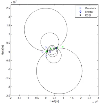
This algorithms shows the moderate accuracy with lower computation than the first one. However, it requires a proper initial point. If not the location may diverge or converge on the wrong location. In this paper, therefore, the method for getting the initial point is proposed through this paper. The key point is that the initial point is obtained by using RSS algorithms with the expected range of the radiated power of the non-cooperative emitter. For an example, in the case of using 4 receivers, there are 6 Apollonius circles and 2 intersection points as shown in Fig. 2. And then, it is possible

to estimate the emitter’s location by assuming the radiated power is from 0.1 mW to 50 mW. Among these results, the nearest location and the farthest location are used for initial point of each intersection points.

The flowchart of the proposed algorithm is given in Fig. 3.

And the criterion or method for selecting one location for both of two intersection points is not covered in this paper.

Fig. 2. Concept of getting initial points from RSSI results.

Fig. 3. Flowchart of the prosed algorithm.

(5)

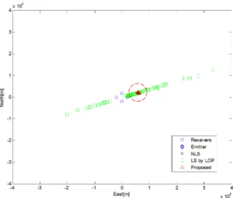
5. SIMULATION

In this section, the location accuracy of each algorithms is analyzed according to the number of receiver, and the number is set as 4, 8, and 12. The distance between the local origin point and each receivers is about 2,000 m, and each receivers are arranged asymmetrically because of the requirements of the LS by LOP algorithm. And one emitter is location at (6000, 2000) which is farther than each receiver’s location. For NLS algorithm, the grid points and size are set to 25 m and 10 m, respectively.

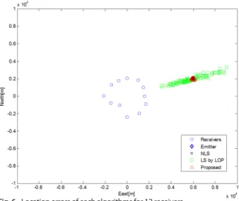
The localization results according to the number of receivers are given in Figs. 4-6, and the localization errors are also given in Table 1.

From these results, it can be checked that the proposed algorithm provide better performance than that of LOP

algorithms which is a general algorithm for linear least squares. Although the proposed algorithm cannot superior to NLS algorithm, that algorithm is hard to process in real- time because it can be only implemented in batch form.

And the errors of all algorithms are reduced as the number of receivers increase. Therefore, the number of the receivers can be determined according to the required performance specification.

6. CONCLUSIONS

A simple and efficient localization algorithm using received signal strength is proposed. The main idea is to determine the initial point of the linearized least squares by using the results of general RSSI algorithm for expected Fig. 4. Location errors of each algorithms for 4 receivers.

Fig. 5. Location errors of each algorithms for 8 receivers.

(6)

range of the transmitted power. And. it is shown by simulations that the proposed algorithm provide better location accuracy than that of LOP algorithm and it can be applied in a real-time processing whereas NLS algorithm has difficulties in real-time processing. Therefore, it can be expected that this algorithm will be easily used for RF interference localization.

REFERENCES

Alam, N., Balaie, A. T., & Dempster, A. G. 2010, Dynamic Path Loss Exponent and Distance Estimation in a Vehicular Network using Doppler Effect and Received Signal Strength, in Proc. of IEEE 72nd Vehicular Technology Conference - Fall, 6-9 Sept. 2010, Ottawa: Canada, pp.1- 5. https://doi.org/10.1109/VETECF.2010.5594457 Caffery, J. J. 2000, A New Approach to the Geometry

of TOA Location, in Proc. of IEEE 52nd Vehicular Technology Conference - Fall, 24-28 Sept. 2000, Boston: USA, pp.1943-1949. https://doi.org/10.1109/

VETECF.2000.886153

Cheung, K. W., So, H. C., Ma, W.-K., & Chan, Y. T. 2003, Received Signal Strength Based Mobile Positioning via Constrained Weighted Least Squares, in Proc. of 2003 IEEE International Conference on Acoustics, Speech, and Signal Processing, 6-10 April 2003, Hong Kong: China, pp.137-140. https://doi.org/10.1109/

ICASSP.2003.1199887

Hata, M. 1980, Empirical formula for propagation loss in land mobile radio services, IEEE Transactions on Vehicular Technology, 29, 317-325. https://doi.

org/10.1109/T-VT.1980.23859

Jackson, B. R., Wang, S., & Inkol, R. 2011, Received Signal Strength Difference Emitter Geolocation Least Squares Algorithm Comparison, Proc. of IEEE Canadian Conference on Electrical and Computer Engineering, 8-11 May 2011, Niagara Falls: Canada, pp.1113-1118.

https://doi.org/10.1109/CCECE.2011.6030635

Juang, R.-T., Lin, D.-B., & Lin, H.-P. 2006, Hybrid SADOA/

TDOA Location Estimation Scheme for Wireless Communication Systems, in Proc. of IEEE 63rd Vehicular Technology Conference, 7-10 May 2006, Melbourne: Australia, pp.1053-1057. https://doi.

org/10.1109/VETECS.2006.1682995

Wang, S. & Inkol, R. 2011, A Near-optimal Least Squares Solution to Received Signal Strength Difference based Geolocation, in Proc. of 2011 IEEE International Conference on Acoustics, Speech and Signal Processing, 22-27 May 2011, Prague: Czech Republic, pp.2600-2604.

https://doi.org/10.1109/ICASSP.2011.5947017

Weiss, A. J. 2003, On the accuracy of a cellular location system based on RSS measurements, IEEE Transactions on Vehicular Technology, 52, 1508-1518. https://doi.

org/10.1109/TVT.2003.819613

Xia, H. H. 1996, An analytical model for predicting path loss in urban and suburban environments, in Proc. of 7th IEEE International Symposium on Personal, Indoor and Mobile Radio Communications, 18-18 Oct. 1996, Taipei: Taiwan, pp.19-23. https://doi.org/10.1109/

PIMRC.1996.567505 Fig. 6. Location errors of each algorithms for 12 receivers.

Table 1. Comparison of the location errors for each algorithms.

Non-linear LS (m) LS by LOP (m) Proposed (m) 4 Receivers

8 Receivers 12 Receivers

23.59 21.24 20.60

3965.62 2562.44 1509.36

154.27 108.35 89.40

(7)

Deok Won Lim received the B.S and Ph.D degrees in the Department of Electronics Engineering from Chungnam National University, Korea in 2004 and 2011, respectively. He is now working in Korea Aerospace Research Institute. His research interests include GNSS receiver design and anti-jamming technologies.

Jae-Hee Seo received M.S. degrees in electronics engineering from Kyungpook Nation- al University, Korea in 2015. Since 2016, he has been working at Korea Aerospace Research Institute. His research interests include GNSS, indoor navigation, RTLS and LBS .

Sebum Chun received a Ph.D degree in aerospace engineering at Konkuk university in 2008. His research interests include GNSS, non-linear filter and indoor navigation.