2003, Vol. 14, No.4 pp. 965∼974
Incremental Multi-classification by Least Squares Support Vector Machine1)
Kwangsik Oh2) ․ Jooyong Shim3) ․ Daehak Kim4)
Abstract
In this paper we propose an incremental classification of multi-class data set by LS-SVM. By encoding the output variable in the training data set appropriately, we obtain a new specific output vectors for the training data sets. Then, online LS-SVM is applied on each newly encoded output vectors. Proposed method will enable the computation cost to be reduced and the training to be performed incrementally. With the incremental formulation of an inverse matrix, the current information and new input data are used for building another new inverse matrix for the estimation of the optimal bias and lagrange multipliers. Computational difficulties of large scale matrix inversion can be avoided. Performance of proposed method are shown via numerical studies and compared with artificial neural network.
Keywords : Multi-class, LS-SVM, Incremental training, Neural network, Classification, Inverse matrix.
1. Introduction
In recent years, chiefly as a consequence of the development of the electronic computer, considerable advances have been made in the practical application of statistical classification analysis. Classification analysis is a multivariate technique concerned with assigning an object into one of several possible categories.
Machine learning based method like support vector machine(SVM) introduced by Vapnik(1995, 1998) are competing modern technology to traditional statistical methods. Despite of many successful application of SVM in the area of statistical 1) This research was supported by Catholic University of Daegu research Grants in 2003.
2) Professor, Department of Statistical Information, Catholic University of Daegu,
3) Adjucnt Professor, Department of Statistical Information, Catholic University of Daegu, 4) Professor, Department of Statistical Information, Catholic University of Daegu,
classification, a modified version of SVM was proposed by Suykens and Vanderwalle(1999a) in a least squares sense(LS-SVM) for classification. In LS-SVM the solution is given by a linear system instead of a quadratic programming problem. But their LS-SVM algorithm has also some limit. The data should be trained in batch form, which is not suited to the real application such as an online system identification and control. So incremental online training for the classification is needed urgently in real data application where the data come in sequentially.
On the while Ahmed et al.(1999) has brought forth an incremental training algorithm for SVM classification. The basic idea is that only the support vectors are preserved and these support vectors plus the new coming data are used for training again. The main drawback is that the training is not exactly incremented.
It is approximately incremental and the Lagrange multipliers corresponding to the support vectors are not updated incrementally. Cauwenberghs and Poggio(2001) proposed the exact incremental and decremental training for SVM classification.
Friess and Cristianini (1998) proposed a sequential gradient method for SVM, where the main problem is that the training is not convergent quickly. Scholkopf et al.(1995) used voting scheme methods based on combining many binary class SVM's for the multi-class pattern recognition. Weston and Watson(1999) generalized the binary class SVM to the multi-class SVM without using combination of binary class SVM's. Suykens and Vandewalle(1999b) proposed a multi-class LS-SVM corresponding to a set of linear equations composed of newly encoded training data sets.
In this paper we propose the exact online(incremental) training method for multi-class LS-SVM. We devide the set of linear equations composed of newly encoded training data sets into a specific number of sets of linear equations and apply online LS-SVM on each set of linear equations.
The rest of paper is organized as follows. In Section 2, we examine the multi-classification method based on LS-SVM. In Section 3, we propose the incremental multi-class LS-SVM. In Section 4 we perform the numerical studies with real data sets. Finally we have concluding remarks in Section 5.
2. Multi-classification by LS-SVM
For the classification of multi-class data sets, let us denote the given training data set of N observation by {yi, xi}, i = 1,…,N. Here xi is a multivariate input and yi is a single output which can takes a value between 0 and q-1, where q is the number of classes. For the binary class case, the output can takes only two values like 0 and 1.
For given class number q, we can always find a number m which satisfies
q∈[ 2m - 1+1, 2m]. In order to use LS-SVM for multi-classification, we transform the output yi, i = 1,…,N into a row vector y( i)' = ( yi1,…,yim) of m dimension where yik satisfies yi= ∑m
k = 1yik2k - 1. Actually yik, i = 1,…,N, k = 1,…,m is 0 or 1. With these transformed vectors y( i)' ,i = 1,…,N, we can construct a matrix Y of size N ×m , that is, i-th row of Y is y( i)' which consists of 0's or 1's corresponding to the output yi. And then, we have another transformation which makes the elements of the matrix Y of 0's into -1's. This transformation can make us to apply the binary classification procedure by LS-SVM to multi-classification. Column vectors of Y is expressed as y( k),k = 1,…,m to avoid confusion. So the matrix Y can be represented as
Y = ( y( 1), y( 2)…, y( m))=
ꀌ
ꀘ
︳︳
︳︳
︳︳
︳︳
︳︳
ꀍ
ꀙ
︳︳
︳︳
︳︳
︳︳
︳︳ y( 1)' y( 2)'
… y( N)'
= ꀌ
ꀘ
︳︳
︳︳
︳︳
︳︳
︳
ꀍ
ꀙ
︳︳
︳︳
︳︳
︳︳
︳ y11 y12 … y1m y21 y22 … y2m
⋯ ⋯ … ⋯ yN1 yN2 … yNm
.
Suykens and Vandewalle(1999b) suggested multi-class LS-SVM based on the formulation
Minimize 1 2 ∑m
k = 1wk' wk + C 2 ∑N
i = 1 ∑m
k = 1e2i,k (1)
over { ωk,bk,ei, k} subject to equality constraints
yi, k( wk' φk( xi) +bk) = 1 -ei, k , i = 1,…,N, k = 1,…,m ,
where wk is a weight vector corresponding to the input vectors xi,i = 1,…,N and kth column vector y( k) of Y. Bias and errors corresponding to the input vectors xi,i = 1,…,N and kth column vector y( k) are denoted by bk and ei, k respectively. φk( xi) is the nonlinear feature mapping function of xi,i = 1,…,N associated with y( k) and C is a regularization parameter. The lagrangian function can be constructed as
L( w k,b k,ei, k: αi, k) = 1
2 wk' w k + C
2 ∑
N i = 1 ∑
m k = 1e2i,k
- ∑
N i = 1 ∑
m
k = 1α i, k {yik( wk' φk( xi)+b k)-1+e i, k} (2)
where αi, k's are the lagrange multipliers. The conditions for optimality are given
by
∂L
∂ wk = 0 → w k=∑
N i = 1 ∑
m
k = 1αi, kφ k( x i),k = 1.…,m
∂L
∂bk = 0 → ∑
N
i = 1αi, kyik= 0,k = 1,…,m
∂L
∂ei.k = 0 → αi, k= C ei, k, i = 1,…,N, k = 1,…,m
∂L
∂αi, k = 0 → yik( wk' φk( xi) + bk)-1+ei, k= 0 , i = 1,…,N, k = 1,…,m
and we have a solution
[Y0mm×m Ω m+CY m'- 1I ][ ]α b = [ ]1 0 . (3)
Here, α = ( α1',…, α m')' and b' = ( b1,b2,…,bm) denote the solutions of (3) and
Ym= Blockdiag { y( 1), y( 2),…, y( m)} = ꀌ
ꀘ
︳︳
︳︳
︳︳
︳︳
︳︳
︳
ꀍ
ꀙ
︳︳
︳︳
︳︳
︳︳
︳︳
︳ y( 1) 0 … 0
0 y( 2) … 0
⋯ ⋯ … ⋯
0 0 … y( m) Nm×m and
Ωm= Blockdiag {Ω ( 1),…,Ω ( m)} = ꀌ
ꀘ
︳︳
︳︳
︳︳
︳︳
︳︳
ꀍ
ꀙ
︳︳
︳︳
︳︳
︳︳
︳︳
Ω ( 1) 0 … 0
0 Ω ( 2) … 0
⋯ ⋯ … ⋯
0 0 … Ω ( m) Nm×Nm
where Ω( k) is a N × N matrix with ( i,j)th element by yikyjkKk( xi, xj), i,j = 1,…,N, k = 1,…,m which is calculated based on kth kernel function Kk(⋅, ⋅). Then for given testing input vector xt, it can be classified as yt by
yt= ∑
m
k = 1ytk×2 k - 1 where
ytk= 0.5×( sign(∑
N
i = 1α i, kyikK k( xi, x t) ) + bk+1), k = 1,…,m.
3. Online multi-class LS-SVM
Assume that we have built LS-SVM model based on the first n data for each data set { y ( i), xi}, i = 1,…,n where y ( i) is defined in the previous section. To apply the multi-class LS-SVM to online LS-SVM, we consider the division of linear system (3) into m sets of linear systems (8).
[
y 0( k) Ω ( k)+ Cy( k) 'k- 1I]
[ bαkk ] = [ ]1 0 ,k = 1,…,m (4)By considering one linear system (3) to m linear systems (4), the regularization parameter Ck,k = 1,…,m can be adjusted for each set of linear equations, which can provide better results than equation (3).
Suppose that now the new data {yn + 1, xn + 1} is coming in. Denote the equation (4) by An( k ) pn( k)= R( k )n , k = 1, …,m , where the subscript n indicates that the current model is based on the first n pairs of data. Then the optimal Lagrange multipliers and bias based on first n pairs of data are obtained from
pn( k)= An( k )- 1R( k )n , k = 1,…,m
such that pn=(bk, α1, k, α2, k,…, αn, k)'. For (n + 1)th pairs of data, we have pn + 1( k)= An +1( k) -1R( k)n+1 , k = 1,…,m (5) where k = 1,…,m
An + 1( k) - 1= [Ad( k)n1' ud1]- 1, (6)
u = Kk( x n + 1, x n + 1)+ 1
Ck, R( k)n + 1= [R1 ( k)n ]
and
d1= {y1ky( n + 1)kKk( x 1, x n + 1) ,…, ynky ( n + 1)kKk( x n, x n + 1) }' for k = 1,…,m. We have two famous inverse equations for matrix
A = [AA2111 AA2212]
A- 1=[[A21[ A-A11-A21A- 11211AA- 12212]A- 1- 121A]- 121A- 111 A- 111[AA1222[A-A21A21A- 122- 111AA12-A12]- 122]- 1] (7)
and
(A+BCD) - 1= A- 1- A - 1B ( C- 1+ DA- 1B )- 1DA- 1 (8) According to (7), the equation (6) can be changed into
A( k )n + 1
- 1= [Ad( k )n1' ud 1] - 1
=ꀎ ꀚ
︳︳
︳︳
ꀏ
ꀛ
︳︳
︳︳ [ A( k )n - 1
u d 1d 1']- 1 A( k )n
- 1 d 1[ d 1' A( k )n
- 1 d 1- u]- 1 [ d 1' A( k )n - 1 d 1- u]- 1d 1' A( k )n - 1 [u - d 1' A ( k )n - 1d 1']- 1
(9)
for k = 1,…,m. Applying the equation (8) to the upper left submatrix in the equation(9), we have
[A( k )n - 1
u d1 d1' ]
- 1
= A( k )n - 1- A( k )n - 1 d1 [- u + d1' A( k )n - 1 d1] - 1 d1' A( k )n - 1
(10)
for k = 1,…,m. Let δ ( k)= [ u - d1' A( k)n
- 1 d1]- 1 then the equation (6) can be changed into
A( k )n + 1- 1=[ A0( k )n - 1 0 1 ]+ δ( k )[ A( k )n- 1- 1 d1][ d1' A( k )n - 1 - 1] (11)
for k = 1,…,m. With the equation (11) the inversion of matrix is computed through an incremental form, which avoids expensive inversion operation. Thus we can compute the equation (5) to get the optimal lagrange multipliers α1, k, α2, k,…, αn + 1, k and bias bk for k = 1,…,m based on A( k )n and {yn + 1, xn + 1} without inverting A( k)n+1 directly. Then we get the online formulation for multi-class LS-SVM for each new data set. After completion of new coming data set, we have trained multi-class LS-SVM which can be used to the classification of testing data sets.
4. Numerical studies
In this section we illustrate the performance of proposed online multi-classification algorithm. The two famous data sets - Iris data set and Wine data set were considered for the comparison. The gaussian kernel function with
several values of bandwidth parameter σ is used. The regularization parameter Ck's of equation (4) were chosen appropriately by prior guess and used for the numerical studies. The data points are added one by one and the corresponding the lagrange multipliers and bias are updated every time for the incremental formulation in the equation (5).
The Iris data set is the benchmarking data set for the classification. It consists of four measurements made on each of 150 flowers. There are three pattern classes - Virginica, Setosa and Versicolor - corresponding to three different types of Iris. Since the number of classes q is 3, m should be equal to 2. So the two linear systems of (4) is used for proposed online multi-class LS-SVM. In this case, the reference set consists of 150 feature vectors in 4 dimension. Each of the data point is assigned to one of three classes. In this numerical study, we choose 75 data points of the three classes - Virginica, Setosa and Versicolor - for the training data set and remained 75 data points for the testing data set.
To visualize the training data set we restrict two features which contain the most information of the class, the petal width and petal length. The scatter plot of training data points is shown in figure 1. From the scatter plot of Iris data, we can conjecture class 2 and class 3 can't be separated by linear hyper plane which leads to the use of gaussian kernel function.
Figure 1. Iris data set : The scatter of training data points(Left) and testing data points(Right) for two selected features.
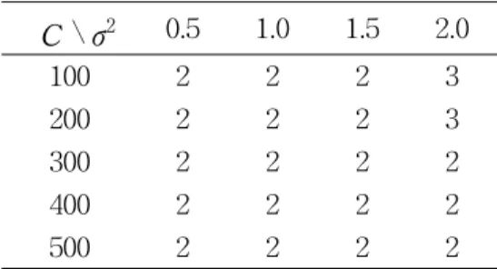
Table 1 shows the number of misclassifications for testing data set by the proposed online multi-class LS-SVM. Proposed method and batch method explained in section 2 provide exactly same results for the Iris data set, so we gave the result from the proposed method only. Comparisons are made according to the 4 values of σ2 in gaussian kernel function and 5 values of regularization parameter C. In this case we used same regularization parameters C=C 1= C2 in order to compare both methods.
Table 1. The number of misclassifications for Iris data set C \ σ2 0.5 1.0 1.5 2.0
100 2 2 2 3
200 2 2 2 3
300 2 2 2 2
400 2 2 2 2
500 2 2 2 2
For another comparison of proposed method, we employ the artificial neural networks(ANN) of 1 hidden layer with 5, 10, 15, 20 and 25 nodes, respectively.
We performed 20 runs for each ANN and obtained the smallest number of misclassifications and the largest number of misclassifications, which are shown in table 2. As seen in table 2 ANN does not provide stable solutions on this data set and all of the numbers of misclassifications are larger than those obtained by the proposed online multi-class LS-SVM in average sense.
Table 2. The number of misclassifications for the Iris data by ANN.
number\node 5 10 15 20 25
smallest 1 5 3 2 4
largest 9 16 13 9 17
average 5 10.5 8 5.5 10.5
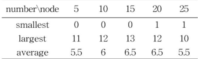
The Wine data set is found in UCI machine learning repository, of which data are the results of a chemical analysis of wines grown in the same region in Italy but derived from three different cultivars. An analysis determined the quantities of 13 constituents found in each of the three types of wines, class 1 , 2 and 3 with 59, 71 and 48 data points, respectively. We divide the wine data set into two parts - 128 data points for the training data set and 58 data points for the testing data set. Similarly to the iris data we use gaussian kernel function. And ANNs of 1
hidden layer with 5, 10, 15, 20 and 25 nodes, respectively. are employed for the comparison. Table 3 shows the number of misclassifications for testing data set by the online multi-class LS-SVM and the batch multi-class LS SVM according to the values of σ2 and C=C 1= C2. Both methods provide exactly same results also in Wine data set. As seen in table 4 ANN does not provide stable solutions on this data set also and most of numbers of misclassifications are larger than those obtained by the multi-class LS-SVM.
Table 3. The number of misclassifications for Wine data set.
C \ σ2 0.5 1.0 1.5 2.0
100 2 1 0 0
200 2 1 1 1
300 2 2 3 3
400 2 2 3 3
500 2 2 3 3
Table 4. The number of misclassifications for Wine data set by ANN.
number\node 5 10 15 20 25
smallest 0 0 0 1 1
largest 11 12 13 12 10
average 5.5 6 6.5 6.5 5.5
5. Concluding Remarks
We proposed an online multi-classification by LS-SVM. Performance of proposed method are compared with batch multi-classification by LS-SVM and artificial neural networks, respectively. Through the numerical studies we found that the proposed algorithm derives the satisfying results, whose performance is reasonably well without running a large scale matrix inversion operation, which is attractive approach to modelling the training of large data set. Also hyper parameters in the propose method can be adjusted more efficiently than in a batch method proposed by Suykens and Vandewalle(1999b).
References
1. Ahmed, S. N., Liu, H. and Sung, K. K. (1999). Incremental Learning
with Support Vector Machines, International Joint Conference on Artificial Intelligence (IJCAI99), Workshop on Support Vector Machines, Stockholm, Sweden.
2. Cauwenberghs, G. and Poggio, T. (2001). Incremental and Decremental Support Vector Machine Learning, In Leen, T. K., Dietterich, T. G. and Tresp, V., editors, Advances in Neural Information Processing Systems 13 : 409-415, MIT Press.
3. Friess, T. and Cristianini, N. (1998). The Kernel-Adatron: A Fast and Simple Learning Procedure for support vector machines, Proceeding of the Fifteenth International Conference on Machine Learning (ICML), 188-196.
4. Mercer, J. (1909). Functions of Positive and Negative Type and Their connection with Theory of Integral Equations, Philosophical Transactions of Royal Society, A:415-446.
5. Scholkopf, B., Burge, C. and Vapnik, V. (1995). Extracting Support Data a Given Task. Proceeding of First International Conference on
Know1edge Discovery and Data Mining.
6. Suykens, J.A.K. and Vanderwalle, J. (1999a). Least Square Support Vector Machine Classifier, Neural Processing Letters, 9, 293-300.
7. Suykens J.A.K. and Vandewalle, J.(1999b) Multi-class Least Squares Support Vector Machines, Proceeding of the International Joint
Conference on Neural Networks(IJCNN'99), Washington DC, USA, July.
1999.
8. Suykens J.A.K., De Brabanter J., Lukas L. and Vandewalle J. (2002).
Weighted Least Squares Support Vector Machines: Robustness and Sparse Approximation, Neurocomputing, Special issue on fundamental and information processing aspects of neurocomputing, vol. 48, no. 1-4, 85-105.
9. Vapnik, V. N. (1995). The Nature of Statistical Learning Theory.
Springer, New York.
10. Vapnik, V. N. (1998). Statistical Learning Theory. Springer, New York.
11. Weston, J. and Watson, C.(1999). Support Vector Machines for multi-class Pattern Recognition, Proceeding of the Seventh European Symposium on Artificial Neural Networks.
[ received date : Aug. 2003, accepted date : Oct. 2003 ]