IEG 환경지질연구정보센터

전체 글

(1)Min-max correlation-based band reduction for edge detection in hyperspectral images Nguyen van Huan and Hakil Kim Image Information Research Center School of Information and Communication Engineering, INHA University {huan, hikim}@vision.inha.ac.kr. Abstract. This paper presents a min-max correlation-based method of selecting significant bands from hyperspectral image for multi-dimensional edge detection. Due to the huge amount of data, the hyperspectral imagery may include information redundancy in highly correlated bands. The proposed method selects a set of significant bands in a recursive process by applying the min-max criterion to the pair-wise correlation coefficients among bands. The edge is then computed using the set of selected bands by considering each pixel as a spectral vector, and then edge magnitude in the direction of the maximum rate of change is computed. The experiments show that the result of edge detection is saturated with the number of bands and usage of all bands may not result in a meaningful edge image. Key words: Band selection, multi-dimensional edge detection, min-max correlation.. I. Introduction Edges show the discontinuities or sharp changes in digital images, both grayscale and color. Edge information is one of the most important features for image processing applications. For hyperspectral images, edge is, even a challenge to define (Koschan and Abidi, 2005), a difficult problem due to the information redundancy and the confliction between bands. As the number of bands increases, hyperspectral data is more redundant in information content. Band selection algorithms are developed for the aim to select a limited number of bands out of hundred bands so that the band subset can maximize the overall information content. The basis is based on the hypothesis that not every band in the hyperspectral image contains the same amount of information. In the remote sensing literature, band selection methods have been commonly developed for the image visualization purpose (Beaudemin and Fung, 2001). Due to the huge size of the hyperspectral images, encompassment of all bands for edge computation on the one hand is computationally and timely expensive, and on the other hand may degrade the edge detection results because of the data. redundancy. Chavez, et al. (1982) proposed the Optimum Index Factor (OIF) that can be expanded to select p bands from N available bands by maximizing p. OIFp = ∑ m. 1/2 ii. i =1. ⎡ p −1 p ⎤ ⎢ ∑ ∑ abs (cij ) ⎥ ⎣ i =1 j =i +1 ⎦. −1. (1). where mii is the variance of ith band and. abs (cij ) is the absolute correlation between ith and jth bands. However, the OIF is impractical to apply to select a subset of bands for edge detection when p and N are large since we need to compute the above N! index for C Np = combinations. Sheffield p !( N − p)! (1985) proposed a method based on the size of the hyperspace spanned by the data bands. The criterion for selection is to maximize the following index (2) SI = M p. p× p. where M p× p is the determinant of the covariance matrix of the subset of size p. Again, the index is only applicable to a small number of p. This study proposes a fast and computable method for selecting a subset of p bands among N available bands, no matter how large they are. As the. - 239 -.

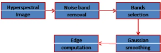
(2) correlation coefficient is a robust quantity for indicating the information redundancy, the proposed method operates on the correlation coefficient matrix of the hyperspectral image. The edge detection considers each pixel as a vector in the spectral domain in order to find the direction of maximum change; then the edge amplitude is computed in that direction.. II. Edge detection The edge is computed as the diagram shown in Figure 1, where Noise band removal uses the method in (Huan, 2009).. Figure 1. Diagram of edge computation. II.1 Bands selection for edge detection The correlation coefficient is a statistically mathematic quantity that measures the strength and direction of a linear relationship between two random variables. The correlation coefficient between a pair of bands is defined as follows: w. h. cij = ∑∑ ( x[i ]mn − x[i ])( x[ j ]mn − x[ j ]), m =1 n =1. rij =. cij cii c jj. },. Assume that the selected band list includes k bands Lk = { Bi1 , Bi 2 ,..., Bik } , then the (k+1)th band is recursively added by the following min-max criterion:. {. κ ∈N − Lk λ∈Lk. II.2. Edge image detection A straightforward way to compute the edge image is to compute the edge of individual bands, then combine them up. However, this method has the weakness of the localization variability in each individual band (Dinh et al., 2009). Another preeminent way is to consider each pixel as a vector in the spectral image, and then performs the edge detection in this domain. In this study, the Di Zenzo (1986) edge detection for multiple images which is a vector based approach is extended to compute the hyperspectral edge image. The main idea is to find the direction for a point x for which its vector in the spectral domain has the maximum rate of change. Let Lk = { Bi1 , Bi 2 ,..., Bik } is the selected band list for edge computation; two derivative vectors u and v are defined as. 0 < i, j < N. u. =. v. =. ∂ B i1 b ∂ x ∂ B i1 b ∂ y. Let the quantities. between ith and jth bands, respectively. The proposed method considers each band as a random variable, and then selects the set of bands that minimizes the correlation to each others. Let RN × N = {rij } denote the correlation coefficient matrix, the first step of the proposed method is to find the band pair which has the lowest correlation:. {. L2 = Bi , B j | rij = min r. }. (4) The above criterion assures that the two selected bands have the least redundancy. The new band is added to the selected band list in a recursive manner. r∈R. (5). The above min-max rule guarantees that the newly added band has a low correlation to the all bands in the list.. (3). where w, h are the spatial size of the image, and cij , rij are the correlation and correlation coefficient. }. Lk +1 = Lk , Bi ( k +1) | min max(rκλ ). 1. + ... +. 1. + ... +. ∂ B ik b ∂ x ∂ B ik b ∂ y. γ xx , γ yy , γ xy be. k. (6) k. defined in terms. of the dot product of these vectors, as follows: 2 2 ∂Bk ∂ B1 γ xx = u .u = + ... + ∂x ∂x. γ. yy. ∂ B1 = v .v = ∂y. 2. ∂Bk + ... + ∂y. 2. (7). ∂Bk ∂Bk ∂ B1 ∂ B1 + ... + x y ∂ ∂ ∂x ∂y The direction of the maximum change rate at a pixel (x, y) is given by (Di Zenzo, 1986): (8) ⎡ 2γ ⎤ 1. - 240 -. γ xy = u . v =. θ = tan −1 ⎢ 2. xy. ⎥ ⎢⎣ (γ xx − γ yy ) ⎥⎦.

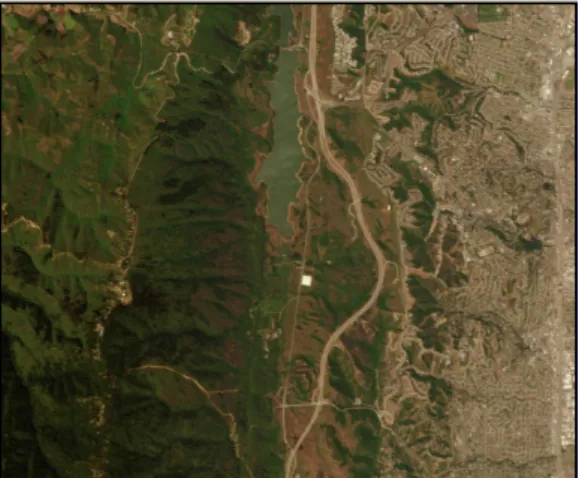
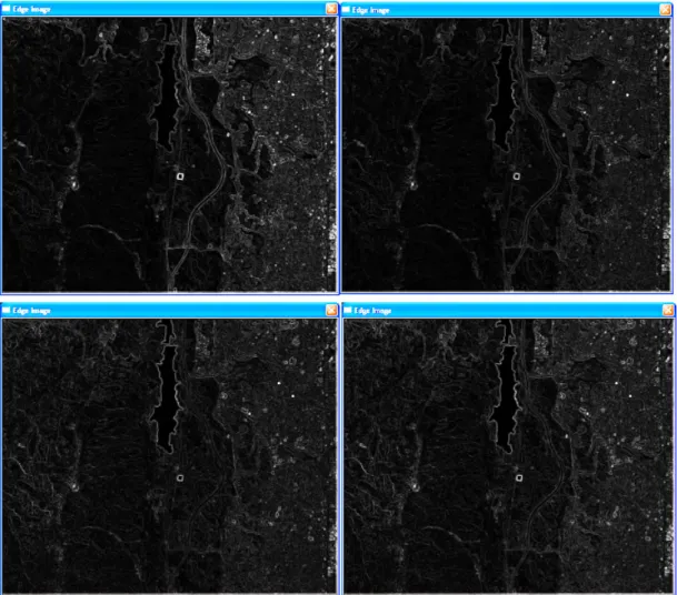
(3) The amplitude of the change at that direction is given by: 1. ⎤ ⎪⎫ 2 ⎪⎧ 1 ⎡(γ xx + γ yy ) Γ(θ ) = ⎨ ⎢ ⎥⎬ ⎩⎪ 2 ⎢⎣ + (γ xx − γ yy ) cos 2θ + 2γ xy sin 2θ ⎥⎦ ⎭⎪. (9). In this study, the implementation of the partial derivatives required in the Eq [6] uses the Sobel mask (Sobel, 1968).. III. Experiments III.1 Datasets The dataset used in this experiment is a part of an AVIRIS free sample data, acquired on July 5, 1996 over an area of Southeast Washington D.C. (AVIRIS data). The data has 224 bands of size 510 rows × 612 columns, ranging from 374 to 2,503 nm wavelengths.. where Ek denotes the edge image using k bands and M, N are the spatial sizes of the hyperspectral image. Table 1 shows the values of this quantity using different numbers of bands used in edge computation. The experimental results in Fig. 3 below show that the edge image using a small number of bands contains the strong edge with a loss of the weak edges. It is more distinctive to reveal the object shape. As the number of bands involved in edge detection increases, the edge image looks "busy". Also, the results of using 10, 15 and 20 bands shows a small difference from the Fig. 2 as well as the RMSE, indicating that the edge image is saturated at some number of bands. Table 1. The RMSE using different number of bands in edge computation. 3 5 10 15 20. 3 0 -. 5 91.34 0 -. 10 168.21 155.08 0 -. 15 135.34 128.92 36.55 0 -. 20 137.575 137.388 38.00 15.28 0. IV. Conclusions. Figure 2: Color display of the used AVIRIS image. III.2. Experimental results In order to show the effectiveness of the band selection method and the edge results using different numbers of bands, the proposed method is applied to select subsets of bands of different band numbers. In this paper, the results of using 3, 5, 10 and 20 bands are shown in Fig. 3 below. In order to quantitatively describe the difference between two edge images, the root-mean-square error (RMSE) is computed as. erms = ⎡ 1 ⎢ ⎣ MN. M −1 N −1. ∑ ∑ ⎡⎣ E ( x, y) − E ( x, y) ⎤⎦ i. x =0 y =0. j. 2. ⎤ ⎥ ⎦. 1 2. (10). This paper presents a min-max rule to select significant bands for multi-dimensional edge detection. Due to the huge amount of information and redundancy, band selection algorithms are crucial in hyperspectral image processing. The edge image is computed using the set of selected bands by considering each pixel in the hyperspectral image as a vector in spectral domain. The experiments show that the band selection for edge detection is needed for hyperspectral in terms of saving the computational time as well as improvement of the meaningfulness of the result. Further works will try to define mathematical evaluation and compare to other methods.. Acknowledgement This research was supported by the Agency for Defense Development, Korea, through the Image Information Research Center at Korea Advanced Institute of Science & Technology. - 241 -.

(4) Figure 3. Grayscale results of edge detection using different number of bands: 3 bands (top-left), 5 bands (top-right), 10 bands (bottom-left), and 20 bands (bottom-right). (The image is enhanced for a better visualization).. References. Scandinavian Conferences on Image Analysis, LNCS 5575, pp. 580–587, 2009. Huan, N.V., Hakil, K., 2009. Noisy band removal using band correlation in hyperspectral images, Korean Journal of Remote Sensing, Vol. 25, No. 3, pp 263270 Koschan, A. and Abidi, M., 2005. Detection and Classification of Edges in Color Images, Signal Processing Magazine, Special Issue on Color Image Processing, Vol. 22, No. 1, pp. 64-73. Sheffield, C., 1985. Selecting band combinations from multispectral data, Photogrammetric Engineering 6. Remote Sensing, 51(6): pp. 681-687. Sobel, I., Feldman, G., 1968. A 3x3 Isotropic Gradient Operator for Image Processing. Presented at the Stanford Artificial Project. AVIRIS data available online at http://aviris.jpl.nasa.gov/html/aviris.freedata.html Beaudemin, M., and Fung, K.B. 2001. On statistical band selection for image visualization, Photogrammetric Engineering & Remote Sensing, 67(5): pp. 571–574. Chavez, P.S., Jr., Berlin, G.L. and Sowers, L.B. 1982. Statistical method for selecting Landsat MSS ratios, Journal of Applied Photographic Engineering, 8(1):pp. 23-30. Di Zenzo, S., 1986. A note on the gradient of a multi-image. Computer Vision, Graphics, and Image Processing, pp. 116–125. Dinh V. C., Raimund Leitner, Pavel Paclik and Robert P. W. Duin: A Clustering Based Method for Edge Detection in Hyperspectral Images.. - 242 -.

(5)