韓 國 水 資 源 學 會 論 文 集 第41卷 第1號․2008年 1月
pp. 27~34
Strack의 단일 포텐셜 해석해를 이용한 해안지하수 개발가능량 평가
Assessment of Available Coastal Groundwater Resources Using Strack’s Single-potential Analytical Solution
최 뢰* / 이 창 해** / 박 남 식***
Cui, Lei / Lee, Chang Hae / Park, Namsik
...
Abstract
Groundwater development in coastal areas induces saltwater intrusion. In many cases amount of groundwater resources available for development is limited by a pre-specified limit of additional saltwater intrusion. In this paper a simple equation is developed to assess available groundwater resources which depends on the constraint of acceptable additional saltwater intrusion. Strack's single-potential analytical solution is used to derive the equation. Available groundwater increases as more additional intrusion is allowed. However, critical points limit both the maximum pumping rate and the allowed saltwater intrusion limit. The equation is presented in the form of design curves from which the maximum pumping rate can be read off quickly. The equation and the design curves are suitable for preliminary estimation of available groundwater resources in coastal areas.
keywords : saltwater intrusion, available groundwater resources, design curves, Strack's single- potential analytical solution
...
요 지
해안 지역의 관정에서 지하수를 개발하면 해수가 침투하며 많은 경우 대상 지역의 지하수 개발가능량은 허용될 수 있는 추가 해수침투 거리로 제한된다. 본 연구에서는 주어진 허용 추가 해수침투 거리를 위배하지 않는 해안 지 역의 지하수 개발가능량을 평가할 수 있는 수식을 개발하였다. 개발가능량 산정을 위한 수식의 유도에는 Strack의 단일 포텐셜 해석해가 이용되었다. 개발가능량은 추가 허용 해수침투 거리를 늘림에 따라 증가하지만 critical point 로 인하여 최대값이 제한된다. 개발가능량 산정식은 설계곡선의 형태로도 제시되었다. 유도된 식 또는 설계곡선을 이용하면 기본계획 단계의 지하수 개발가능량을 쉽게 평가할 수 있다.
핵심용어 : 해수침투, 지하수 개발가능량, 설계곡선, Strack's 단일 포텐셜 해석해
* 동아대학교 공과대학 토목공학부 박사과정
Ph.D. Student, School of Civil Engineering, Dong-A University, Busan, 604-714, Korea (e-mail: [email protected])
** 대진대학교 공과대학 환경공학과 부교수
Associate Professor, Dept. of Environmental Engrg., Daejin University, Gyeonggi-do, 487-711, Korea (e-mail: [email protected])
*** 동아대학교 공과대학 토목공학부 교수
Professor, School of Civil Engineering, Dong-A University, Busan, 604-714, Korea (교신저자) (e-mail: [email protected])
DOI: 10.3741/JKWRA.2008.41.1.027
1. INTRODUCTION
Groundwater is an important source of freshwater in coastal areas in many regions around the world.
Inadequate development or management may cause depletion or contamination of groundwater resources.
Thus, accurate estimation of available groundwater resources is the important first step for rational management. In Korea groundwater resources available for development is generally estimated as a certain percentage of total recharge. Generally the same percentage is used regardless of site-specific characteristics. However, groundwater available for development depends strongly not only on natural conditions such as recharge rate, hydrogeologic variables, etc. but also on design parameters such as number and location of wells.
In coastal areas saltwater intrusion phenomenon is an additional, if not most important, feature that needs to be considered for proper development of groundwater. In general groundwater development induces saltwater intrusion. In many design problems for groundwater development there may be a preset limit for tolerable saltwater intrusion. For these problems the maximum pumping rates need to be determined without violating the constraint on saltwater intrusion. For wells distributed in an irregular pattern a combined approach of simulation and optimization techniques is required to obtain the solution.
Saltwater intrusion phenomenon is complex and accurate simulation is difficult. Nevertheless modeling techniques are available. The techniques can be grouped into two categories; (1) The density- dependent flow-and-transport approach (Voss, 1984;
Kim, 1996) accounts for effects of solute concentration on the fluid density. This is by far the most physically accurate method. However, data requirement and computational efforts are expensive.
(2) The sharp-interface approach (Reilly and Goodman, 1987) assumes immiscible freshwater and saltwater separated by abrupt (sharp) interface. As the transition zone between two waters is ignored, it is not as accurate as the aforementioned approach.
The approach is suitable for regional groundwater
development. Reilly and Goodman (1987) compared their solutions with those obtained by Bennett et al.(1968), based on the sharp interface approximation supported the validity of the sharp-interface assumption for analyzing the behavior of systems with thin saltwater-freshwater transition zone. Park et al. (2004) found that salt concentrations can be estimated with reasonable accuracy. Therefore the sharp-interface approach is a viable alternative to the flow-and-transport approach.
There are a number of optimization techniques available to be used in conjunction with simulation methods. The genetic algorithm is one of the popular global optimization methods. The method is heuristic but is capable of escaping local extrema, which may be difficult for derivative-based optimization method.
The simulation-optimization technique is the most versatile tool to determine optimal pumping rates with constraints. Park and Hong (2006) developed a general-purpose computer program to solve design problems. Although versatile, the technique requires large amount of computing time. To reduce the computing time for repeated simulations, required for optimization, the sharp-interface analytical solution developed by Strack (1976) can be used when simplifying assumptions are applicable (Cheng et al., 2000; Park and Aral, 2003).
In this work a direct solution of the maximum pumping rate is obtained for design problems, without the use of an optimization technique. Strack's solution is commonly used to determine the response of an intruding saltwater wedge to groundwater pumping. In this work his solution is recast in such a way that the maximum pumping rate, subject to a preset limit on saltwater intrusion, can be determined directly. The solution is simple, but comprehensive in that practically all relevant parameters are accounted for. The solution is also presented as design curves.
Direct solution is possible only when wells are distributed in a regular pattern. In practice such distribution of pumping wells may not be possible.
Therefore, the method proposed herein must be regarded as a tool for preliminary assessment of potential groundwater resources in coastal areas.
2. MAXIMUM PUMPING RATE 2.1 Strack's Single Potential Solution
Strack (1976) developed an analytic solution for interface problems in coastal aquifer. A single governing potential equation was used to solve the problems across two zones of the costal aquifer.
(Fig. 1)
Strack(1976) defined a potential for confined and unconfined aquifers as follows:
For confined aquifers
for zone 1 (1)
for zone 2 (2)
For unconfined aquifers
for zone 1 (3)
for zone 2 (4)
where is the freshwater head, is the confined aquifer thickness, is the elevation of mean sea level above the aquifer base, and s, which equal to , is the density ratio of the saltwater and freshwater,
and are the saltwater and freshwater densities, respectively.
The potential functions satisfy the Laplace equation
∇ (5)
The interface location can be defined through the use of proper boundary conditions:
For confined aquifers:
(6)
For unconfined aquifers:
(7)
The toe of the saltwater wedge is located at
, from Eqs. (6) and (7)
(a) a confined aquifer
(b) an unconfined aquifer
Fig. 1. Cross-sectional Views of Coastal Aquifers
For confined aquifers:
(8)
For unconfined aquifers:
(9)
The freshwater potential for multiple wells, in an aquifer with uniform flow, can be obtained using the method of superposition(Strack, 1976; Cheng et. al, 2000)
(10)
where is the pumping rate from well ; (, ) is well coordinate.
By combining Eq. (8) or Eq. (9) and Eq. (10), we can get equations for toe positions:
For confined aquifers:
(11)
For unconfined aquifers:
(12)
2.2 Basic Dimensionless Equations
Determination of the maximum pumping rates which would limit the saltwater intrusion to a pre-specified location when wells are arbitrarily distributed is generally a nonlinear optimization problem, which requires a complex optimization technique. However, when wells are placed in a regular pattern maximum pumping rates can be determined without optimization technique. To this end the following conditions are assumed regarding the well placement:
① The number of wells is an odd number, equal or greater than three;
② Wells are aligned in the parallel direction to the coastline;
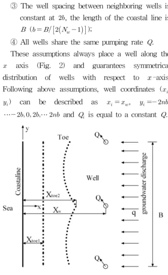
③ The well spacing between neighboring wells is constant at , the length of the coastal line is
( );
④ All wells share the same pumping rate .
These assumptions always place a well along the
axis (Fig. 2) and guarantees symmetrical distribution of wells with respect to -axis.
Following above assumptions, well coordinates (,
) can be described as ,
⋯ ⋯ and is equal to a constant .
Fig. 2. Plan View of Pre-development Toe (Xtoe1) and Post-development Toe in Response to Pumping from Three Wells
From Eqs. (11) and (12), they are very similar and can be combined into one equation for both aquifer types. We define two variables, and :
For confined aquifers: and For unconfined aquifers: and Then the universal equation is obtained as follow:
(13)
Eq. (13) identifies toe coordinates (, ) when
equally spaced wells are pumping at . Since the wells are distributed symmetrically with respect to the
axis, it is clear from the superposition principle that the maximum intrusion of saltwater wedge occurs
along the axis. Since the maximum intrusion occurs along the axis, it is straightforward to determine the desired maximum pumping rate while limiting the saltwater intrusion to a pre-specified location (say,
). The desired maximum pumping rate can be obtained by solving for after substituting and
in Eq. (13). When wells are arbitrarily distributed, the maximum intrusion location is not known and thus, the maximum pumping rate cannot be determined directly. The simulation and optimization approach is needed.
Prior to groundwater development, fresh ground- water discharge and intruding saltwater is in equilibrium. For this condition the toe location can be obtained by setting in Eq. (13). The pre-development toe position is
(14)
Eq. (13) is normalized using the following dimensionless variables:
(15a)
(15b)
(15c)
(15d)
where is the dimensionless pumping rate, is the well position, and is the dimensionless well spacing.
Dimensionless form of Eq. (13) with and
:
(16) The Eq. (16) can be solved for dimensionless
pumping rate:
(17)
Eq. (17) determines explicitly the desired pumping rate, that would limit the saltwater intrusion to the region defined by ≤ . The pumping rate is a function of three independent variables: the dimensionless predevelopment toe position , the dimensionless post development toe , and the well spacing (or equivalently the number of wells). i.e.
. The density ratio can be considered constant.
The pre-development toe position is determined by natural conditions such as aquifer characteristics of coastal groundwater discharge. The other two variables are design parameters. There may be only certain location to place pumping wells, otherwise allowable maximum intrusion may be determined by preexisting wells that exist near the coastal line.
2.3. Limitation of Maximum Pumping Rate Eq. (17) shows that the dimensionless pumping rate is proportional to additional intrusion length
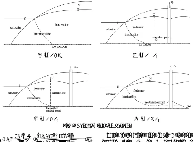
. Therefore, by allowing more intrusion more groundwater can be developed. It is true to some extent Fig. 3(a) and (b). But increase in pumping rates is limited by a critical point(Strack, 1976).
The critical point is defined as a point where stagnation point M induced by the pumping and the toe of the interface coincide, shown in Fig. 3(c). The pumping rate caused the two points coincide is called the critical pumping rate . When the pumping rate
is increased even slightly from the critical pumping rate, the saltwater would contaminate the well Fig.
3(d). Therefore, the maximum pumping rate is limited by , and the pre-specified limit of saltwater intrusion ( ) is also limited by the critical point.
The equation for the critical points can be obtained by requiring that the stagnation point (, 0) to correspond to toe point. We defined additional dimensionless variables for critical intrusion toe point (, 0) as:
M
toe position interface line
freshwater saltwater
stagnation point
M M
Q1
saltwater
toe position interface line
freshwater
(a) for (b) for
stagnation line M
Qmax
saltwater
toe position (critical point) freshwater
interface line
toe
no stagnation point M
Q3
saltwater
freshwater interface line
(c) for (d) for Fig. 3. Saltwater Intrusion Patterns
(18)
3. DESIGN CURVES-DESIRED PUMPING RATES
Eqs. (17) and (18) provide complete information on
subject to . However the maximum pumping rate limited by the critical point is not evident. When these equations are cast in the form of design curves, the limit posed by the critical points can be made obvious. Since the pumping rate is a function of three independent variables, we need to set one variable to derive design curves in a plane.
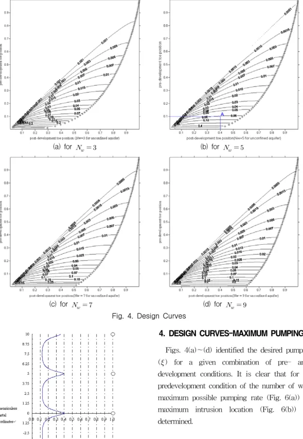
In this section, design curves for the designed pumping rate are presented as a function of pre- and post development toe positions when the number of wells are 3 (Fig. 4(a)), 5 (Fig. 4(b)), 7 (Fig. 4(c)), and 9 (Fig. 4(d)). The figures shows two trends as more well are used:
(1) For a given set of pre and post development conditions, pumping rate for an individual well is decreasing.
(2) More intrusion is allowed without contami- nating the pumping wells.
Values of the contour lines in Fig. 4 represents the pumping rates () for a combination of a predevelopment of toe position () and a maximum allowable post‐development toe position (). The region above the line is invalid since the desired development toe position must be less than the pre-development toe position. The ‘+’ symbols indicate the critical pints, therefore, the region below the curve marked by ‘+’ is also invalid. The curve represents the maximum pumping rates and the maximum allowable toe positions as dictated by critical points. In other words, for a given predevelopment toe position, intersection of the curve and a horizontal line, passing through the given predevelopment toe position, depicts the maximum pumping rate and the maximum saltwater intrusion location that would not contaminate the wells.
Fig. 5 illustrates the example toe position for the case of ( = 0.1, = 0.4; point A in Fig. 4(b)). In this case, the design curves yields the dimensionless pumping rate to be ≈ . As we can see from the figure the maximum saltwater intrusion position is limited by 0.4, as desired.
(a) for (b) for
(c) for (d) for Fig. 4. Design Curves
Fig. 5. Example toe position for point (depicted in Fig. 4(b))]
4. DESIGN CURVES-MAXIMUM PUMPING RATE Figs. 4(a)~(d) identified the desired pumping rate () for a given combination of pre- and post development conditions. It is clear that for a given predevelopment condition of the number of wells, the maximum possible pumping rate (Fig. 6(a)) and the maximum intrusion location (Fig. 6(b)) can be determined.
5. CONCLUSION
A simple method is proposed to estimate potential groundwater resources in coastal areas. Pumping rates can be determined for a given set of hydrogeologic and operational conditions. Practically all the relevant variables are accounted for in estimating the pumping rates, making the method
-0.6 -0.1 0.4 0.9 LOG10 (well spacing)
0.1 0.2 0.3 0.4 0.5 0.6 0.7 0.8 0.9
Pre-development toe position
-0.6 -0.1 0.4 0.9
Log10 (well spacing) 0.1
0.2 0.3 0.4 0.5 0.6 0.7 0.8 0.9
Pre-development toe position
(a) critical post‐development toe positions (b) maximum pumping rates Fig. 6. Maximum Values
comprehensive. Variables considered are: the toe locations before and after groundwater development, hydrogeologic parameters such as hydraulic conductivity, aquifer thickness, and coastal ground- water discharge; and operational variables such as allowable maximum intrusion length, number and location of pumping wells.
To certain extent the available groundwater, pumping can be increased by allowing more saltwater intrusion. However, the maximum saltwater intrusion is limited by so-called critical points that lie between the pre-development toe and the pumping well. This point then identifies the maximum pumping rate.
Design curves are presented for the pumping rates as a function of pre and post development toe positions, maximum pumping rates and maximum intrusion locations as functions of pre development toe position and well spacing.
As with other analytical solutions the equation derived theoretically in this work needs to be validated against field observations. Future study is desired.
Acknowledgement
This research was supported by a grant (code#
3-3-3) from Sustainable Water Resources Research Center of 21st Century Frontier Research Program.
References
Bennett, G.D., Mundorff, M.J., and Hussain, S.A.
(1968). "Electric-analog studies of brine coning beneath freshwater wells in the Punjab Region West Pakistan." U.S. Geol. Surv. Water-Supply Paper, 1608-J .
Cheng, A.H.D., Halhal, D., Naji, A., and Ouazar, D.
(2000). "Pumping optimization in saltwater intruded coastal aquifers", Water Resources Research, Vol. 36, No. 8, pp. 2155-2166
Kim, J.M. (1996). A fully coupled model for saturated‐unsaturated fluid flow in deformable porous and fractured media. Ph.D. Dissertation, Pennsylvania State University, University Park, Pennsylvania, pp. 201
Park, C.-H., Aral, M.M., (2003). "Multi-objective optimization of pumping rates and well placement in coastal aquifers", Journal of Hydrology, v. 290, No. 1-2, pp. 80-99 .
Park, N.S., Bhopanam, N.K., Hong, S.H., Han, S.Y.
(2004). "Sand-tank experimental studies on saltwater intrusion phenomena." SWIM18, Cartagena, Spain
Park, N.S. and Hong, S.H. (2006). “Optimization Model for Groundwater Development in Coastal Aquifers.” Advances in Geosciences, Vol. 4, pp.
159-166
Reilly, T.E. and Goodman, A.S., (1987). "Analysis of saltwater upconing beneath a pumping well."
Journal of Hydrology, 89, pp. 169-204
Strack, O.D.L. (1976). “A single‐potential solution for regional interface problems in coastal aquifers.” Water Resources Res., 12, 1165-1174.
Voss, C.I. (1984). A finite‐element simulation model for saturated‐unsaturated, fluid‐density develop- ment groundwater flow with energy transport or chemically‐reactive single species solute transport. U.S. Geological Survey, Water Resources Investigations Report # 84‐4369
(논문번호:07-144/접수:2007.12.11/심사완료:2007.12.18)