1. Introduction
1.1. Research Background and Objective
Because of increasing demands for high energy efficiency in construction and maintenance of buildings, accurate energy performance simulation through building envelopes has become one of the major issues in the architectural design process. Several general purpose computer-aided energy simulation programs have been developed that calculate the hourly heat gain and loss through shaded fenestration systems. However, most of these programs have not been incorporated in the actual building design process.
The major reason is that there is a lack of suitable software to visualize the energy effects with proper graphical presentation methods1). As the fenestration system is still the least efficient component of most residential and commercial buildings, an accurate and easy-to-use computer simulation program for fenestration and shading design is highly desirable. To develop this kind of program, profound and reliable evaluations should be conducted in order to scrutinize the characteristics of solar effects on the transparent surface of buildings.
pISSN 2288-968X, eISSN 2288-9698 http://dx.doi.org/10.12813/kieae.2014.14.4.035
1.2. The Proposed Program of the Research
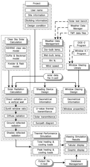
The final objective of this research is to develop program for an energy-efficient fenestration system design, namely the Shaded Fenestration Designer (Fig. 1). This program will be able to calculate the thermal effect of solar radiation and shading devices on a transparent wall and visualize them with proper graphical presentation methods. However, development of this program consists of very complicated procedures which include: 1) thermal performance simulation such as solar geometry, solar radiation calculations, and the incident-angle-dependent heat transfer through multi-pane window systems; 2) window glazing and shading device design; 3) weather data modeling and processing; 4) user interface applying proper graphical presentation techniques; 5) usability tests by architectural designers in order to prove that the program is an adequate design tool showing the solar and shading effects that resulted from architectural design solutions.
As a result, the SFD program (Fig. 1) is being developed as a composite program which includes numerous subroutines and several add-in programs such as the ‘Solar Data Calculator (SolrCalc)’, the ‘Weather Data Converter (Weth-Conv)’, and the
‘Weather Data Displayer (Weth-Disp)’. Images in Fig. 2 are the screen captures of the SFD Weather Data Displayer program showing various display formats for weather data and results of
KIEAE Journal
Korea Institute of Ecological Architecture and Environment
68
1)
An Effective Algorithm for Transmitted Solar Radiation Calculation through Window Glazing on a Clear Day
Oh, John Kie-Whan*
* Corresponding author, Department of Architectural Design, Dongseo University, South Korea. ([email protected])
A B S T R A C T K E Y W O R D
The main objective of this study is to provide an effective algorithm of the transmitted solar radiation calculation through window glazing on a clear day. This algorithm would be used in developing a computer program for fenestration system analysis and shading device design. Various simulation methods have been evaluated to figure out the most accurate and effective procedure in estimation of transmitted solar radiation on a tilted surface on a clear day.
Characteristics of simulated results of each step have been scrutinized by comparing them with measured results of the site as well as results from other simulation programs. Generally, the Duffie & Beckman’s solar calculation method introducing the HDKR anisotropic model provided the most reliable simulation results. The DOE-2 program usually provided over-estimated simulation results. The estimation of extraterrestrial solar radiation and beam normal radiation were conducted pretty accurately. However, the solar radiation either on horizontal surface or on tilted surface involves complicated factors in estimation. Even though the estimation results were close to the real measured data during summer when solar intensity is getting higher, the estimation provided more error when solar intensities were getting weaker. The convex polygon clipping algorithm with homogeneous coordinates was fastest model in calculation of sunlight to shaded area ratio. It could not be applied because of its shape limitation.
ⓒ 2014 KIEAE Journal
Solar radiation calculation,
Analysis of building energy performance, Computerized building energy simulation, Energy-efficient fenestration design, Weather file, Shading analysis
A C C E P TA N C E IN F O Received June 30, 2014
Final revision received August 26, 2014 Accepted August 28, 2014
building performance simulation.
Among these subroutines, the procedures to simulate transmitted solar radiation through window glazing are the core functions in the SFD program. The SolrCalc program (Fig. 3) is an add-in program developed to satisfy this specific objective. The SolrCalc program 1) converts local civil time to local solar time, 2) calculates various solar angles related to the position of the sun for any latitude, longitude, time of day, and day of the year, 3) calculates various kinds of solar radiation on a clear day, such as extraterrestrial solar radiation, beam normal radiation, beam, diffuse, and ground-reflected solar radiation either on a horizontal surface or on a tilted surface, and 4) saves the solar data for a given period in a specific file format (*.SOL). The program provides options for the user to choose one of the solar simulation models.
1.3. Research Process and Method
As it is complicated and difficult to calculate the exact cooling load caused by transmitted solar radiation through multi-pane window glazing, we have to take into account various subtle factors and inappropriate assumptions which can cause us to make mistakes. These mistakes will increase especially when thermal resistance of the target wall is pretty high or the window area is greater than normal. Thus, the traditional heat transfer method using an analytical model, such as the CLTD/SCL/CLF method, the TFM method, or the TETD/TA method, could not be used, because these methods are difficult for an inexperienced person to manipulate and entail high possibility of error. In my previous research, the dynamic analysis method based on a finite difference model applying the HDKR anisotropic sky model and one-minute data was able to greatly reduce the number of calculation errors2). However, this kind of mathematical analysis requires a very accurate definition of boundary conditions and a series of high level calculations. So we need a computerized easy-to-use program that could be greatly helpful to architectural designers who do not have enough knowledge of heat transfer theory that should be incorporated in their ecological architectural design process.
To process this research, equations for transmitted and absorbed (a) Cylindrical sunpath (b)Equidistant sunpath
(c) Psychrometric chart
Fig. 2. The screen image of the SFD Weather Data Displayer (WethDisp) program, displaying simulated solar radiation plotted on sunpath diagrams and measured solar radiation plotted on a psychrometric chart
Fig. 1. Development phases of the Shaded Fenestration Designer (SFD) program, containing the SFD Solar Data Calculator (SolrCalc) program, which is surrounded by a dotted line
solar radiation through window glazing will be analyzed and checked at every stage throughout the whole process of a computerized simulation procedure, in order to arrive at very accurate solar radiation calculation through window glazing. First, accuracy of equations for the calculation of extraterrestrial
radiation and horizontal solar radiation under a clear sky will be analyzed. Then, the process of solar radiation incident on a titled surface will be verified on a comparative basis. Finally, the area ratio of the sunlit area and the shaded area will be evaluated.
Widely-used computerized models for fenestration design and ways of validation and measurement of solar models also need to be reviewed.
2. Calculation of Solar Radiation under Clear Sky
Generally, simulation models for horizontal solar radiation are categorized under three headings: 1) regression models such as the Cloud-cover Radiation Model (CRM)3), the Zhang & Huang Model (ZHM)4), and the Saudi Arabia Model (SAM)5), 2) mechanical models such as the Meteorological Radiation Model (MRM)6) and the Upper –air Humidity Model (UHM)7), and 3) models using high precision measuring instruments or satellite images8). As regression models are required to derive regional coefficients from regressions of long-term measured weather data, it cannot be used in simulation programs using only limited site information. Even though mechanical models do not need regional coefficients, simulation process is more complicated and requires extra weather information that the usual weather station does not measure.
Models using high precision measuring instruments or satellite data certainly are not suitable for the purpose of this study.
Recently the author suggested a hybrid model applying the ZHM for winter season and the CRM for summer season for the sites having critical seasonal weather condition9).
Thus, the simulation models introduced in this program are using the equations suggested by the most widely approved solar models in the United States, including those of the ASHRAE Hand Book of Fundamentals, Diffie & Beckman, and Kreider & Rabl.
2.1. Extraterrestrial Solar Radiation
The extraterrestrial solar radiation () is the solar radiation which would be received on an earth surface if there were no atmosphere. It is quite important in terms of quantity because in many solar radiation models the estimated values of the direct and diffuse radiation on the earth’s surface are derived from it. The radiation emitted by the sun and its spatial relationship to the earth result in a nearly fixed intensity of solar radiation outside the earth’s atmosphere10). Due to the eccentricity of the earth’s orbit, the actual value of extraterrestrial radiation varies by ±3.3%. Thus, the extraterrestrial radiation at the average earth-sun distance, i.e., the solar constant () is used to calculate the actual intensity of the extraterrestrial radiation taking into account seasonal Date
(W/) E. T.
(min.) Declination (degrees) A
(W/) B
(-) C
(-) Jan. 21 1,416 -11.2 -20.0 1,230 0.142 0.058 Feb. 21 1,401 -13.9 -10.8 1,215 0.144 0.060
Mar. 21 1,381 -7.5 0.0 1,186 0.156 0.071
Apr. 21 1,356 1.1 11.6 1,136 0.180 0.097
May 21 1,336 3.3 20.0 1,104 0.196 0.121
June 21 1,326 -1.4 23.45 1,088 0.205 0.134
July 21 1,326 -6.2 20.6 1,085 0.207 0.136
Aug. 21 1,338 -2.4 12.3 1,107 0.201 0.122
Sep. 21 1,359 7.5 0.0 1,152 0.177 0.092
Oct. 21 1,380 15.4 -10.5 1,193 0.160 0.073 Nov. 21 1,405 13.8 -19.8 1,221 0.149 0.063 Dec. 21 1,417 1.6 -23.45 1,234 0.142 0.057 Note: Data are for 21st day of each month during the base year of 1964.
(Reference: ASHRAE, Handbook of Fundamentals, 2005) Table 1. Extraterrestrial solar radiation intensity and related data Fig. 3. Flowchart displaying the main procedures in the SFD Solar Data Calculator (SolrCalc) program
variations.
The ASHRAE handbook11) uses a value of 1,367 W/ for the solar constant. The extraterrestrial radiation varies from a maximum of 1,414 W/ on January 3 to a minimum of 1,323W/ on July 4. ASHRAE provides a table (Table 1) to determine extraterrestrial radiation for the 21st day of each month.
Duffie and Beckman10) used a value of the solar constant rounded to 1,367 W/. A simple equation with accuracy adequate for extraterrestrial radiation can be calculated by
×cos
×
× (1)They also provided a more accurate equation (±0.01%) developed by Spencer such as
cos sin cos sin
× (2)where,
(3)
Kreider and Rabl12) used a slightly larger value of 1,373 W/ for the solar constant and a value of 365.25 for the total days of the year instead of 365 used in the Duffie and Beckman model. Thus, the equation is changed to
×cos
×
× (4)The calculated values of extraterrestrial radiation of each month do not show much difference between these two models, and are close enough to the value of the ASHRAE Handbook. The Kreider and Rabl’s model provides about 0.5% more radiation on average than the Duffie and Beckman’s model, and the value calculated by
the ASHRAE Handbook is between the former two models.
As the value of extraterrestrial radiation depends solely on the day of the year () and is independent of the latitude of the site, and the solar location, as well as the weather conditions, any location on the earth would have the same amount of extraterrestrial solar radiation on the same day of the year. From Table 2, we can see its peak occurs not in summer but in winter solstice (December 21) in the northern hemisphere, and the sun provides the minimum extraterrestrial radiation on summer solstice (June 21).
2.2. Clear Sky Beam Normal Radiation
The intensities of solar radiation reaching the earth’s surface vary during the year because of seasonal changes in the dust and water vapor content of the atmosphere and because of earth-sun distance changes.
In the ASHRAE method, beam normal solar radiation () on a clear day is calculated by
expsin
(5)where = apparent solar radiation at air mass m = 0
= atmospheric extinction coefficient
= solar altitude angle (degrees)
Values of A and B are given in Table 1. These values are not the maximum value for the , but are representative of conditions on cloudless days with a relatively dry and clear atmosphere. Thus, under very clear atmospheres, can be 15% higher than the calculated value that was derived by Equation (5)11).
To develop a more accurate solar simulation model that considers the effects of altitude, visibility, zenith angle, and the Jan 21 Feb 21 Mar 21 Apr 21 May 21 Jun 21 Jul 21 Aug 21 Sep 21 Oct 21 Nov 21 Dec 21
ASHRAE 1,416 1,401 1,381 1,356 1,356 1,326 1,326 1,338 1,359 1,380 1,405 1,417
Duffie & Beckman 1,409 1,395 1,375 1,352 1.333 1,323 1,324 1,338 1,360 1,382 1,402 1,411 Kreider & Rabl 1,415 1,401 1,382 1,358 1,338 1,328 1,330 1,344 1,365 1,388 1,408 1,418
ASHRAE 931
(.6575) 952 (.6795) 959
(.6944) 915 (.6748) 883
(.6512) 864 (.6516) 855
(.6448) 870 (.6502) 905
(.6659) 924 (.6696) 911
(.6484) 908 (.6484)
Duffie &
Beckman
A = 0 km 704 (.4996) 763
(.5470) 806 (.5862) 819
(.6058) 823 (.6174) 819
(.6190) 815 (.6156) 809
(.6046) 789 (.5801) 746
(.5398) 697 (.4971) 673
(.4770) A = 0.2 km 736
(.5224) 793 (.5685) 833
(.6058) 844 (.6243) 847
(.6354) 843 (.6372) 840
(.6344) 834 (.6233) 816
(.6000) 776 (.5615) 730
(.5207) 706 (.5004)
Kreider &
Rabl
A = 0 km 708 (.5004) 768
(.5482) 809 (.5854) 821
(.6046) 826 (.6173) 823
(.6197) 819 (.6158) 812
(.6042) 793 (.5810) 752
(.5418) 702 (.4986) 676
(.4767) A = 0.2 km 740
(.5230) 798 (.5696) 836
(.6049) 847 (.6237) 851
(.6360) 847 (.6378) 843
(.6339) 838 (.6235) 821
(.6015) 782 (.5634) 735
(.5220) 709 (.5000) Note: The calculation is for the case of a non-leap year. The time for solar hour angle is 12:00 noon in local solar time, and the latitude of site is 35oN.
The ASHRAE model is for average cloudless days. For the Duffie & Beckman’s and Kreider & Rabl’s model, the visibility is 23km, and the options for the climate type are set to the midlatitude summer for the period between April 21and September 21 and to the midlatitude winter for the other periods.
The highlighted cells denote either minimum or maximum values for the year in question.
Table 2. Comparisons of extraterrestrial radiation (), clear sky normal beam radiation () ( (W/), and the atmospheric transmittance for beam radiation ()
four climate types of the site, both the Kreider & Rabl and the Duffie & Beckman models introduced ‘atmospheric transmittance’
for estimating the beam radiation transmitted through clear atmospheres, which had been proposed by H. C. Hottel13).
The atmospheric transmittance for beam radiation () is a factor of beam normal radiation to extraterrestrial radiation ( = /
) and is determined by
exp
cos
(6)where, values for , , and k are given in Tables 3 and 4 A = the altitude of the observer in Km
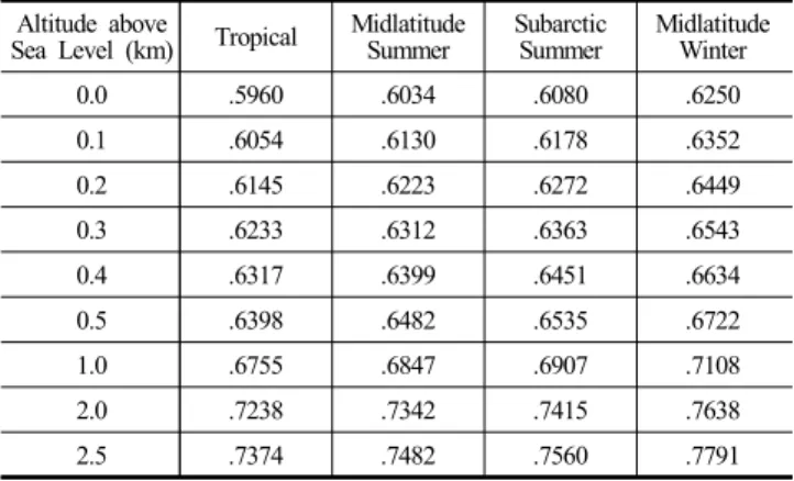
This solar transmittance for a standard atmosphere can be used for any zenith angle and altitude up to 2.5 km. For a clear sky radiation simulation, we can use the values for 23km visibility in Table 4. Table 5 shows simulated values of atmospheric transmittance for different altitudes and climate types. The simulated values ascertained that the climate type is a less critical factor in determining than the altitude of the site. It shows about 20%
difference between the maximum and minimum values for different altitudes, but only about 5% difference for different climate types.
Table 2 shows the values of each month’s extraterrestrial radiation and normal beam radiation on clear days calculated using various solar simulation methods. The application of Hottel’s atmospheric transmittance model makes the simulation results more accurate and more flexible than the ASHRAE clear sky model. Even though the peak of extraterrestrial radiation occurs during the winter, the normal beam radiation reaches its minium value due to the minimum atmospheric transmittance of beam radiation.
However, the ASHRAE clear sky model provides inaccurate results which are very different from results from other models.
The ASHRAE model itself has limited use in a computerized simulation model, because it provides only one representative value for each month. Moreover, as it does not consider the effects of altitude and visibility at the location, a great amount of discrepancy in the estimation of radiation can exist.
Bird and Hulstrom14) have also proposed a simplified clear sky model for direct and diffuse insolation on horizontal surfaces that uses three ‘rigorous radiative transfer codes’. One code is for direct normal irradiance and is called SOLTRAN 4. Two other codes, which include both the beam and the diffuse irradiance, are the BRITE Monte Carlo code and the Dave15) Spherical Harmonics code. A fairly detailed multi-layered atmosphere is constructed by defining important atmospheric parameters at each layer. Each code then uses its own algorithm to solve the radiative transfer problem. When good weather information is not available, the suggested values are given for some input parameters. Although Bird’s model might be more accurate, it is not readily applicable to a computerized model because it requires very detailed weather information such as hourly values for transmittance of aerosol scattering, transmittance of dry air absorptance, amount of ozone, aerosol optical depth, etc.
3. Clear Sky Radiation on a Horizontal Surface
Direct solar radiation on a horizontal surface for a clear day ( ) is determined by beam normal radiation, and the angle between the zenith and the sun. Thus,
cos (7)
Liu & Jordan16) developed an empirical relationship between extraterrestrial radiation and diffuse radiation for clear days. The atmospheric transmittance for diffuse radiation () is the ratio of clear sky diffuse radiation to extraterrestrial radiation on a
Altitude above
Sea Level (km) Tropical Midlatitude
Summer Subarctic
Summer Midlatitude Winter
0.0 .5960 .6034 .6080 .6250
0.1 .6054 .6130 .6178 .6352
0.2 .6145 .6223 .6272 .6449
0.3 .6233 .6312 .6363 .6543
0.4 .6317 .6399 .6451 .6634
0.5 .6398 .6482 .6535 .6722
1.0 .6755 .6847 .6907 .7108
2.0 .7238 .7342 .7415 .7638
2.5 .7374 .7482 .7560 .7791
Note: The calculation is for the case of a non-leap year. The zenith angle is 28o and visibility is 23 km.
Table 5. Simulated values of the atmospheric transmittance for beam radiation ()
23 km Visibility 5 km Visibility
[0.4237-0.00821 (6.0-A)2] [0.2538-0.0063 (6.0-A)2]
[0.5055+0.00595 (6.5-A)2] [0.7678+0.0010 (6.5-A)2]
[0.2711+0.01858 (2.5-A)2] [0.2490+0.0810 (2.5-A)2] (Reference: Hottel, H.C., Solar Energy, 1976)
Table 3. Correction factors for altitude and visibility
Climate Type
23 km Visi. 5 km Visi.
Tropical 0.95 0.92 0.98 1.02
Midlatitude Summer 0.97 0.96 0.99 1.02
Subarctic Summer 0.99 0.98 0.99 1.01
Midlatitude Winter 1.03 1.04 1.01 1.00
(Reference: Hottel, H.C., Solar Energy, 1976) Table 4. Correction factors for climate types
horizontal surface ( = / ) and is calculated by
×cos
(8)
From the above equations diffuse solar radiation on a horizontal surface on a clear day () can be calculated by
× × ×cos (9) Thus, total solar radiation on a horizontal surface on a clear day () is
cos (10) The Equation (10) shows that the total solar radiation on a horizontal surface under clear sky can be calculated only by extraterrestrial radiation (), zenith angle (), and atmospheric transmittance for beam radiation (). However, one can calculate the estimated clear day solar radiation on a horizontal surface if the zenith angle, altitude, and the climate type for the location are given.
Table 6 shows the simulation results of beam, diffuse, and global radiation calculated using the methods of ASHRAE, Duffie &
Beckman, and Kreider & Rabl. As we can expect, the maximum radiation on a horizontal surface reaches its maximum point either in May or in June, and its minimum in December.
4. Clear Sky Radiation on a Tilted Surface
Total solar radiation incident on a tilted surface can be calculated as the sum of beam radiation, diffuse radiation from the sky, and
radiation reflected from various surfaces such as the ground, external shades, and neighboring objects that block the view of the surface. If the view of the surface is blocked from direct sunlight, the total incident beam radiation on a tilted surface ( ) is
∙∙ (11)
where is the tilt factor which is the ratio of the beam radiation component on a tilted surface to that on a horizontal surface, and is the sunlit factor defined by the sunlit area divided by the total surface area. When the incidence angle of direct sunlight () is known,
cos cos
(12)
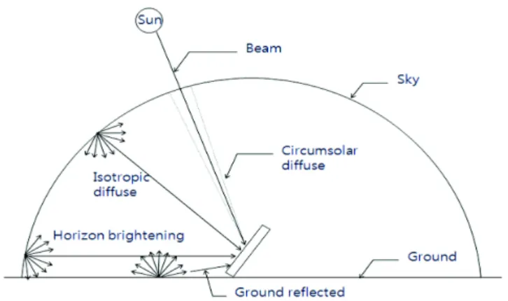
In general, there are two kinds of solar radiation models based upon the method of simulating diffuse solar radiation: an ‘isotropic model’ and an ‘anisotropic model’. In an isotropic sky model, it is assumed that diffuse radiation is isotropic or constant. In other words, the diffuse radiation from the sky is the same regardless of the orientation. However, in an anisotropic sky model, the calculation of the diffuse radiation component on a tilted surface is a little more complicated. Diffuse radiation actually consists of three different components: the ‘isotropic diffuse’ radiation delivered uniformly from the sky hemisphere, the ‘circumsolar diffuse’
radiation scattered around the direct rays of the sun, and the ‘horizon brightening’ which is concentrated near the horizon (Fig. 4).
The Liu and Jordan17) model for diffuse radiation is currently the most widely used. In this model, the solar radiation on a tilted surface () is composed of the beam, the isotropic diffuse, and
Jan 21 Feb 21 Mar 21 Apr 21 May 21 Jun 21 Jul 21 Aug 21 Sep 21 Oct 21 Nov 21 Dec 21
ASHRAE 344 462 570 635 670 673 661 626 549 452 343 294
Duffie &
Beckman
A = 0 km 402 527 656 730 776 781 763 718 627 500 394 352
A = 0.2 km 420 548 679 752 799 804 786 741 649 520 413 370
Kreider &
Rabl
A = 0 km 405 531 658 730 778 784 767 722 633 508 400 354
A = 0.2 km 424 552 680 753 802 807 789 744 655 528 419 371
ASHRAE 85 93 96 98 99 97 96 96 95 94 86 81
Duffie &
Beckman
A = 0 km 100 106 110 112 113 112 112 111 108 104 99 97
A = 0.2 km 95 100 104 105 106 105 105 104 102 98 94 91
Kreider &
Rabl
A = 0 km 100 107 111 113 113 113 112 111 109 105 100 97
A = 0.2 km 95 101 105 106 106 106 105 105 103 99 94 92
ASHRAE 429 555 666 735 767 770 757 722 644 546 429 375
Duffie &
Beckman
A = 0 km 502 633 767 842 889 893 875 829 736 604 493 449
A = 0.2 km 515 648 783 857 905 909 891 845 751 618 506 461
Kreider &
Rabl
A = 0 km 505 638 769 843 892 897 879 833 742 613 500 451
A = 0.2 km 519 653 785 859 908 913 895 849 757 627 513 463
Note: The same condition as Table 5. The highlighted cells denote either minimum or maximum values for the year in question.
Table 6. Comparison of simulated clear sky beam ( ), diffuse ( ), & global ( ) radiation on a horizontal surface (W/)
the ground-reflected radiation. Kreider and Rabl used the simple isotropic model, and suggested the equation for the global irradiance on a titled surface as follows:
cos (13)
where
cos
,
cos , and
= reflectivity of the ground (usually, =0.2)
When vertical surface and the ground in front of the surface is not shaded, the titled surface angle = 90o and Equation (13) becomes simply
cos
(14)
Reindl et al.18) developed an improved anisotropic model called the ‘HDKR model’ by adding a horizon brightening component to the model originally developed by Hay and Davies19) and modified by Klucher20). This model uses an ‘anisotropy index’ to determine the transmittance of the atmosphere for beam radiation. It is assumed that isotropic diffuse radiation from the sky has the same angle as beam radiation. The diffuse radiation on a tilted surface () using the HDKR model is calculated by
cos
(15)where is an anisotropy index and defined by
, and
(16, 17)
Perez et al.21) also developed another anisotropic sky model which considers the zenith angle of the direct beam, cloud clearness, air mass, and the brightness coefficient of the sky.
Diffuse radiation on a tilted surface is again calculated by
cos
sin
(18)where and are circumsolar and horizon brightness coefficients determined by three parameters that describe the sky conditions: the zenith angle, cloud clearness, and brightness. The values of and are calculated from the table for brightness coefficients.
The previous study ascertained that the method developed by Liu and Jordan is less accurate than the anisotropic models22). The model developed by Perez et al. is also difficult to apply in a computer program, because it requires values that weather stations do not usually measure. Thus, the anisotropic model developed by Reindl et al. (i.e., HDKR model) is the most suitable for the calculation of diffuse radiation on a vertical surface.
The ground-reflected solar radiation on a tilted surface () is determined by the total radiation on the horizontal surface (), the view factor of the surface to the ground ( ), and the ground reflectance (). For a surface directly in the front of a collector extending in all directions, the view factor to the ground is
cos.
Generally, in sky radiation model the reflected radiation from the surrounding objects is ignored, because it is much smaller than the reflected radiation from the ground. However, in the case when a large portion of the window surface is blocked by external surfaces, the reflected radiation from these surfaces should be considered.
The total reflected radiation from the surrounding surfaces () can be calculated by the multiple of the solar radiation incident () on the ith surface, the diffuse reflectance() of that surface, and the view factor() from the th surface to the analyzed tilted surface.
Finally, the total solar radiation on a tilted surface () is calculated as the sum of these components. Thus, the total solar radiation on a tilted surface is
cos
cos
(19)For the computerized algorithm of the total solar radiation incident on a tilted surface, Equation (19) was most suitable. In this equation, it is critically important to calculate the incident angles and view factors between glazing and shading objects.
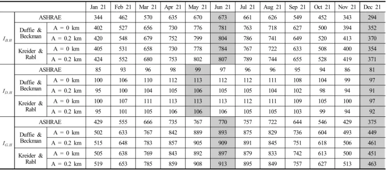
Table 7 shows the simulation results tested for solar radiation on a vertical wall facing 15oSE. It clearly shows the rapid decrease of direct radiation during the summer season (e.g., the value in June 21 is just about 10 % of that in December 21 in Duffie & Beckman model), and almost constant values of diffuse radiation throughout the whole year. However, the reflected radiation increases during the summer season.
Fig. 4. Beam, isotropic diffuse, circumsolar diffuse, horizon brightening, and ground reflected radiation on a tilted surface
5. Calculation of Transmitted & Absorbed Radia- tion through Window Glazing
When the reflection and absorption losses through the glazing are considered, the transmittance () of a single-glazed window can be calculated by applying ray-tracing methods to Fresnel’s equation and Snell’s equation. The total reflection () of unpolarized radiation was calculated using perpendicular (⊥) and parallel (∥) components of unpolarized radiation as follows
⊥ sin
sin
, ║ tan
tan
, (20, 21)
and
⊥ ║ (22)
where and are incident and reflected solar radiation, and and are incidence and refraction angles respectively. The total transmittance () of single-pane glazing can be calculated applying the ray-tracing method to Fresnel’s equations as follow
⊥ ⊥
⊥
⊥ ⊥
, ║ ║ ║
║ ║
,and
⊥ ║ (23, 24, 25)
where ⊥ and ∥ are the perpendicular and parallel components of transmittance of the glazing and is the transmittance of glazing when only absorption losses have been considered. The
value of is defined as,
exp
cos
(26)where = the extinction coefficient
= the thickness of the glazing
The total amount of the transmitted solar radiation through window glazing can be calculated from the above equations.
However, some portion of the transmitted solar radiation will be absorbed by the inside surface and some will be reflected back to the glazing. Thus, for the more accurate estimation of heat gain from the transmitted solar radiation, we need to calculate how much of the transmitted solar radiation is actually absorbed by the inside surfaces. The total solar radiation transmitted through glazing and absorbed by the inside surfaces can be calculated using the ‘transmittance-absorptance product ()’ as follows
cos
cos
∑ (27)Applying the same ray-tracing method here the () can be calculated by
∞
(28)
where is the reflectance of the glazing for the diffuse radiation
Jan 21 Feb 21 Mar 21 Apr 21 May 21 Jun 21 Jul 21 Aug 21 Sep 21 Oct 21 Nov 21 Dec 21
ASHRAE 475 459 385 265 173 133 164 253 372 445 470 463
Duffie &
Beckman
A = 0 km 522 480 414 207 106 56 86 196 341 423 545 533
A = 0.2 km 547 509 428 214 109 58 89 202 353 461 571 560
Kreider &
Rabl
A = 0 km 524 491 417 213 109 56 88 199 342 443 547 534
A = 0.2 km 548 510 431 219 112 58 91 205 354 461 573 561
ASHRAE 42 47 48 50 49 49 48 48 47 47 43 40
Duffie &
Beckman
A = 0 km 50 53 55 56 55 56 55 55 54 51 50 48
A = 0.2 km 47 50 52 52 53 52 52 52 51 49 47 46
Kreider &
Rabl
A = 0 km 50 53 55 56 56 56 56 55 54 52 50 48
A = 0.2 km 47 50 52 52 53 53 52 52 51 49 47 46
ASHRAE 43 56 67 74 77 77 76 72 64 55 43 38
Duffie &
Beckman
A = 0 km 49 62 76 81 86 86 84 80 71 58 49 44
A = 0.2 km 51 64 77 83 88 88 86 81 72 59 51 46
Kreider &
Rabl
A = 0 km 50 63 76 81 86 87 85 80 71 59 50 45
A = 0.2 km 51 64 78 83 88 88 86 82 73 60 51 46
ASHRAE 560 561 500 389 299 258 288 373 483 546 556 541
Duffie &
Beckman
A = 0 km 621 595 545 344 247 198 225 331 466 532 644 625
A = 0.2 km 645 623 557 349 250 198 227 335 476 569 669 652
Kreider &
Rabl
A = 0 km 624 607 548 350 251 199 229 334 467 554 647 627
A = 0.2 km 646 624 561 354 253 199 229 339 478 570 671 653
Note: The time for solar hour angle is 12:00 noon in local solar time, and the latitude of site is 35oN. The building azimuth is 15oSE. The highlighted cells denote either minimum or maximum values for the year in question.
Table 7. Comparison of simulated clear sky beam ( ), diffuse ( ), reflected ( ) & global ( ) radiation on a vertical wall (W/)
from the inside surface and is the absorptance of the inside surface. This solar absorptance is dependent on the angle of incidence of the radiation striking the surface, and can be calculated as a function of the normal incidence for a flat black surface as follows
× ×
× ×
(29)
where is the normal incidence for a flat black surface and is the incidence angle on the surface.
Fig 5 shows the solar test bench, which was used for the validation of the transmitted solar radiation calculation as well as the glazing transmittance test. Besides this solar test bench, a physical model was constructed and used to collect the real measured transmitted solar radiation though window glazing. For more detailed description of physical model and validation of the simulation model, please refer to the previous research22).
6. Calculation of Sunlight to Shaded Area Ratio
To calculate very accurately the transmitted and absorbed solar radiation through glazing, the shading analysis must be included in the computerized calculation process.
Several methods have been developed for the calculation of the sunlit and shaded area of a window. One of the simplest methods is an algorithm with ‘discrete element analysis with grids’ (Fig. 6).
This method was first developed by Groth and Lokmanheim and used in the earlier version of DOE-223) and BLAST24). In this method, the receiving surface is divided into a two dimensional grid. The center point of each element is then tested by a shading projection algorithm to determine whether it is in sunlit or shaded
areas. The sum of the sunlit or shaded grid elements is then used to obtain the sunlit and shaded fraction, respectively. Unfortunately, this method can require excessive processing time for higher resolution. Furthermore, it can only solve rectangular plane surfaces, which means that non-rectangular surfaces must be represented with combinations of rectangular planes.
In the recent version of DOE-2, an ‘improved bar-method’ (Fig.
7) was developed that uses bars instead of grids for a discrete element analysis. This method increased both the speed and accuracy of the calculation. However, the processing speed is still dependent on the desired accuracy and the method still has similar geometrical limitations as the grid method, although not as restrictive.
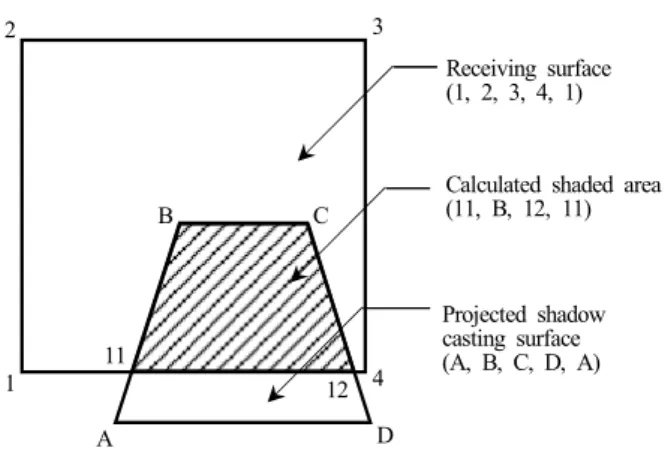
The most recent version of BLAST uses a ‘convex polygon clipping algorithm with homogeneous coordinates’ (Fig. 8) developed by Walton25). In Walton’s method, the dimensional Cartesian coordinates are transformed into dimensional homogeneous coordinates. For example, a point given by two dimensional coordinates (, ) is represented by three dimensional coordinates (, , ), where h is an arbitrary number. After the coordinate transformation, the algorithm finds the vertices of one polygon within the other and visa versa. Then, the intersecting points of the boundary of both polygons are determined. These
Projected shadow casting surface Calculated shaded area
Receiving surface with discrete bars
(a) (b) (c) (d)
(e) (f) (g)
Fig. 5. Configuration of solar test bench (a) multi-pyranometer array with an artificial horizon, (b) Eppley normal incidence pyrheliometer, (c) horizontal solar transmittance test box, (d) shadow band, (e) Eppley shadow band pyranometer, (f) Eppley precision spectral pyranometer, (g) test stand for calibrating pyranometers
Receiving surface with discrete grids
Calculated shaded area
Projected shadow casting surface
Fig. 6. Calculation of the shaded area using discrete grid elements