Seasonal variation of the zooplankton community of Gamak Bay, Korea

changes in phytoplankton standing stocks, and with the combined effects of regional climatology and local hydrog- raphy.

Gamak Bay is surrounded by Yeosu city and Dolsan Island, Korea. Since the 1990s, it has been exposed to en- vironmental pollution, such as eutrophication, harmful algal blooms, and decomposition of sediments caused by increased urban sewage discharged from the metropoli- tan city of new town development and by-products from fishery farming (Lee and Kim 2008). The sediment has been organically enriched and contaminated with anthro-

https://doi.org/10.11626/KJEB.2020.38.2.231

INTRODUCTION

Coastal ecosystems are zones of high productivity and biodiversity. The hydrographic regime within coastal bays is complex, and includes estuarine circulation, formation of fronts, internal waves and wind, tidal mixing, and vertical density gradients (Cembella et al. 2005). Zooplankton is a key component in coastal ecosystems, primarily because of their important role in material and energy fluxes from phytoplankton to higher trophic levels (David et al. 2006).

In general, zooplankton density has been associated with

Original article

Seasonal variation of the zooplankton community of Gamak Bay, Korea

Seong Yong Moon*, Hee Yong Kim and Hyun Ju Oh

South Sea Fisheries Research Institute, National Institute of Fisheries Science, Yeosu 59780, Republic of Korea

1

Ocean Climate and Ecology Research Division, National Institute of Fisheries Science, Busan 46083, Republic of Korea

Korean J. Environ. Biol.

38(2) : 231-247 (2020) ISSN 1226-9999 (print) ISSN 2287-7851 (online)

* Corresponding author Seong Yong Moon Tel. 061-690-8944 E-mail. [email protected]

Received: 16 February 2020 Revised: 25 April 2020

Revision accepted: 27 April 2020

Abstract: The seasonal variation in the zooplankton community and hydrographic con-

ditions were examined in three regions (inner, central, and outer regions) of Gamak Bay, Korea. Zooplankton samples were collected over a period of 12 months from January to December 2006. The hydrographical parameters of temperature, salinity, chlorophyll-a concentrations, dissolved oxygen, and chemical oxygen demand were measured. The total zooplankton density varied from 411 to 58,485 ind. m

, with peaks in early summer.

A total of 65 taxa accounted for approximately 86.9% of the annual mean zooplankton den sity: Noctiluca scintillans (30.9%) Paracalanus parvus s. l. (24.3%), Acartia omorii (11.9

%), Eurytemora pacifica (5.7%), cladocerans (4.1%), cirriped larvae (3.8%), Oithona similis

(3.7%), and Pseudevedne tergestina (2.5%). Copepods dominated numerically throughout the year and comprised 54.3% of the total zooplankton. Most of the dominant copepods showed a well-defined seasonal pattern. The density and diversity of zooplankton in Gamak Bay were influenced by the hydrographic environment that was subject to sig ni fi- cant spatial and temporal variations. Multivariate statistics showed that seasonal temper- ature was the most significant predictor of zooplankton taxa, density, and diversity, as well as the density of dominant taxa. Our results suggest that fluctuations in the zooplankton pop u la tions, particularly copepods, followed progressive increments in the temperature and COD concentrations.

Keywords: Gamak Bay, zooplankton community, copepods, Noctiluca scintillans, tem-

perature, COD

pogenic pollutants in the northern area of Gamak Bay. For the reason, the polluted sediments have been dredged for a long time from 2001 to 2006 (Seo et al. 2012). Neverthe- less, hypoxia and/or anoxia continuously occurs during summer when the water column is stratified, and bottom waters are isolated from oxygen input in the northern re- gion of Gamak Bay (Kim et al. 2006; Lee and Moon 2006;

Moon et al. 2006a).

Study of zooplankton is important for better understand- ing of the functioning of coastal ecosystems (Chisholm and Roff 1990; Leandro et al. 2007). Most information on zooplankton in Gamak Bay is based on seasonal sam- pling of an adjacent region since the 1980s (Shim and Ro 1982; Soh et al. 2002; Moon et al. 2006a, b; Moon et al.

2009; Kang et al. 2018). A previous study on zooplankton populations in Gamak Bay described seasonal communi- ty, taxonomic composition, and density at inner region of Gamak Bay (Soh et al. 2002; Moon et al. 2006b). Studies of zooplankton communities are strongly influenced by temperature, salinity, dissolved oxygen, and phytoplankton standing stocks of different water masses in Gamak Bay (Soh et al. 2002; Moon et al. 2006b). However, estimates of spatial and temporal variation of zooplankton density have not been reported for Gamak Bay.

The major objective of this study was to evaluate zoo- plankton variability in spatial and temporal terms in re- lation to physical and chemical factors and biotic factors along inner, central, and outer regions of Gamak Bay. The study examines the spatial and temporal patterns of density by dominant taxonomic groups.

MATERIALS AND METHODS 1. Experimental methods

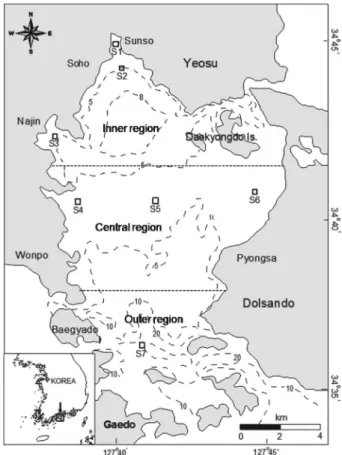
Seasonal variation of the zooplankton community and hydrographic conditions were examined at three regions (inner, central, and outer regions) of Gamak Bay, Korea (Fig. 1). Filtered sampling was conducted at 7 fixed stations monthly from January to December 2006 in Gamak Bay, Korea. Temperature, salinity, and dissolved oxygen (DO) were measured using YSI 6600 model water quality system calibrated against Winkler titrations (Winkler et al. 2003).

Water samples were collected with a 5 L Niskin-type sam- pler from 1 m below the surface and 1 m above the bottom at each station. Chemical oxygen demand (COD) was ana- lyzed by Alkali method (The Oceanographic Society of Ja-

pan 1980). For the determination of total chl-a concentra- tions, a 500 mL sub-sample was gently filtered (vacuum < 5 cm Hg) through a GF/F filter (Whatman Inc., USA), and extracted with 90% acetone for 24 h in dark. Chl-a con- centrations were determined fluorometrically by Cary 300 model (Varian Co., USA) spectrophotometry (Parsons et al. 1984).

Zooplankton samples were collected by vertical hauls from the bottom to the surface using a conical net (0.45 m mouth diameter, 200 μm mesh). The net was fitted with a flow meter (Model 438115, Hydro-bios, Germany) to determine the amount of water filtered during each tow.

Zooplankton samples were immediately preserved in sea- water-buffered formaldehyde (5% final concentrations) for enumeration and identification. In laboratory, subsamples were made with a Folsom plankton splitter, and dispensed into Bogorov-Rass counting chambers. Taxonomic com- position within each zooplankton group was then deter- mined. Copepods were identified, and counted to species level if possible. Subsamples for identification and enu-

Fig. 1. Map showing the sampling stations in Gamak Bay from

January to December 2006.

meration were at least 10% of total samples. Zooplankton identification was made to the lowest taxon possible, and counts were made by Olympus SZ-40 stereomicroscopy.

Zooplankton density was expressed as the number of indi- viduals per cubic meter (ind. m

). The Shannon-Weaver diversity index (H′; Shannon and Weaver 1963) was calcu- lated using PRIMER (Clarke and Warwick 2001).

2. Statistical analysis

Two-way analysis of variance (ANOVA) was used to ex- amine the spatial and temporal differences, i.e., between the sampling stations and between months in all hydrographic variables, zooplankton taxa, density, and diversity. Two-way ANOVA was used also to analyze the spatial and temporal variations in each dominant species. Zooplankton density data were natural log transformed to meet assumptions of normality (i.e., to minimize the influence of highly abun- dant species). Small deviations from normality or homoge- neity after transformation were accepted, because ANOVA is considered to be robust to such violations (Underwood 1997). Pearson’s correlation coefficient was calculated to characterize the relationships of different hydrographic variables, zooplankton taxon, density, and diversity. The effects of hydrographical factors on the seasonal and spatial variations of zooplankton were analyzed by multiple regres- sions based on correlation coefficients among parameters obtained from the sampling data. Parameters selected for all statistical analyses were mean temperature, salinity, DO, COD, and chl-a concentrations within the surface and bot- tom depths from January to December, 2006. All statistical analyses were conducted using SPSS ver. 18.0 for windows.

RESULTS

1. Hydrographic environment

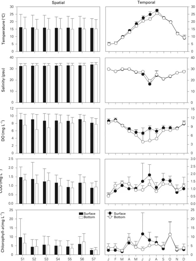
Figure 2 shows the spatial and temporal variations in hy- drographical parameters. Temperature did not show signif- icant spatial variation. However, surface layer (F ⁼ 346.72, p < 0.001) and bottom layer (F = 402.07, p < 0.001) showed significant seasonal variations. The mean tempera- ture values ranged ((4.8±1.2) to (27.2±0.9))°C in Janu- ary to August, respectively. Surface and bottom salinity did not show significant spatial variation. The lowest value of mean salinity of (28.3±1.0) psu was recorded in July while the highest of (35.0±0.2) psu was found in April. Surface (F ⁼ 54.75, p < 0.001) and bottom (F ⁼ 61.74, p < 0.001)

salinity showed significant seasonal variations. Surface and bottom DO concentrations did not show significant spatial variations. The highest mean DO concentration of (9.1±

1.3) mg L

was recorded at S6. It did not significantly differ between stations. Surface (F ⁼ 19.05, p < 0.001) and bot- tom (F = 18.91, p < 0.001) DO concentrations showed sig- nificant seasonal variation. The lowest value at the bottom of (3.9±2.4) mg L

was recorded in June, while the high- est value at the surface of (11.2±0.6) mg L

was found in February. The highest value of mean COD concentrations of (1.4±0.6) mg L

was recorded at S1 surface. Spatial variability of surface temperature was not significant. How- ever, that of bottom temperature was significant (F ⁼ 2.47, p = 0.031). Surface (F = 4.87, p < 0.001) and bottom (F ⁼ 5.04, p < 0.001) COD concentrations showed signif- icant seasonal variations, with the lowest value of (0.5±

0.2) mg L

recorded in January, while the highest value de- tected at the surface of (1.9±0.7) mg L

was in June. The highest value of chl-a concentrations of (9.7±10.4) μg L

was recorded at S1 surface. It decreased slightly toward the bay. The lowest value of chl-a concentrations of (2.5±0.9) μg L

was recorded at S7 surface. The spatial variability of chl-a concentrations was not significant. However, the seasonal variabilities of surface (F = 4.14, p < 0.001) and bottom (F ⁼ 4.67, p < 0.001) chl-a concentrations were significant. The lowest value of chl-a concentrations was recorded at surface of (2.5±0.9) μg L

in December, while the highest value was found at surface (11.6±11.8) μg L

in July.

The results of Pearson’s correlation analysis showed some significant associations among the number of species, den- sity, diversity index (H′), and hydrographical factors (Table 1). Temperature showed significant correlations with all dependent and independent values. Salinity showed signif- icant positive correlations with DO, but significant nega- tive correlations with COD, chl-a concentrations, number of taxa, and density of zooplankton. DO concentrations had significant negative correlation with number of species, while COD concentrations had significant positive correla- tions with chl-a concentrations, number of taxa, and densi- ty of zooplankton.

2. Zooplankton community structure, density and diversity

A total of 65 taxa of zooplankton were recorded. Of zoo-

plankton identified to species level, number of individuals

of Noctiluca scintillans (mean 1,082 ind. m

), Paracalanus

Fig. 2. Spatial and seasonal variations of the hydrographical factors from January to December 2006 in Gamak Bay. The data are means

with SD indicated by the error bars.

Spatial Temporal

Temperature(°C)Salinity(psu)DO(mg L-1 )COD(mg L-1 ) Chlorophyll-a(mg L-1 ) _Surface

Bottom Surface

Bottom 30

25 20 15 10 5 0

30 25 20 15 10 5 0 40

30

20

10

0

40

30

20

10

0 12

10 8 6 4 2 0

15 12 9 6 3 0 3.0 2.5 2.0 1.5 1.0 0.5 0.0 25 20 15 10 5 0 2.5

2.0 1.5 1.0 0.5 0.0 25 20 15 10 5 0

S1 S2 S3 S4 S5 S6 S7 J F M A M J J A S O N D

parvus s. l. (mean 851 ind. m

), Acartia omorii (mean 418 ind. m

), Eurytemora pacifica (mean 199 ind. m

), cirriped larvae (mean 133 ind. m

), Oithona similis (mean 130 ind.

m

), and Pseudevadne tergestina (mean 88 ind. m

) were found (Table 2). Noctiluca scintillans was the overwhelm- ingly dominant species based on overall density contri- bution. This species alone contributed as high as 30.9%

of the total zooplankton density. The low temperature as- semblage was dominated by only a few species, such as E.

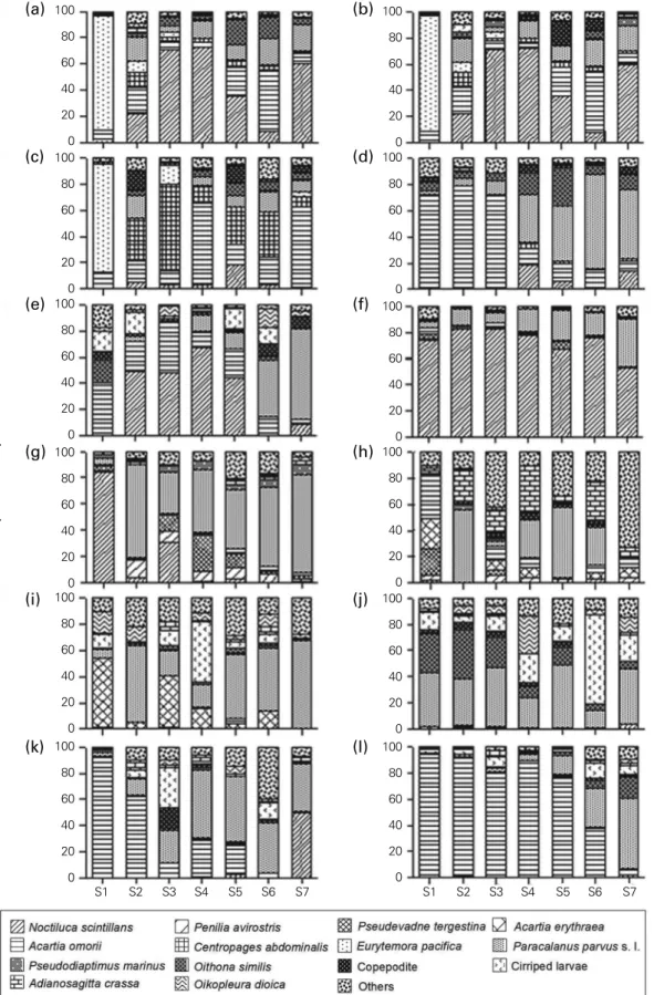
pacifica, A. omorii, and C. abdominalis. At the inner region (S1), mainly E. pacifica was found during January to March while the high-temperature assemblage was mainly domi- nated by P. parvus s. l. during almost the entire study peri- od (Fig. 3). In contrast, the outer region was dominated by

Table 1. Pearson’s correlation coefficient between different environmental factors, taxon density and diversity collected over the spatial

and temporal scales from Gamak Bay

Temperature Salinity DO COD Chl-a Taxon Density

Salinity -0.713** -

DO -0.701** 0.218* -

COD 0.502** -0.623** ns -

Chl-a 0.437** -0.374** ns 0.403** -

Taxon 0.510** -0.492** -0.358** 0.331** ns -

Density 0.247* -0.407** ns 0.460** ns 0.321** -

H ′ 0.281** ns ns ns ns ns -0.218*

*p<0.05, **p<0.01, ns is not significant.

Table 2. Mean abundance of the total zooplankton

(ind. m

), the number of species, species diversity, and dominant taxa (mean±SD). SD is the standard deviation and RA is the relative abundance (%)

Species Minimum Maximum Mean±SD RA

Noctiluca scintillans 4 39,215 1,082±4,456 30.9

Paracalanus parvus s. l. 10 7,117 851±1,214 24.3

Acartia omorii 2 4,671 418±739 12.0

Eurytemora pacifica 4 5,189 199±884 5.7

Cirriped larvae 2 2,341 133±329 3.8

Oithona similis 3 2,489 130±305 3.7

Pseudevadne tergestina 9 2,788 88±367 2.5

Oikopleura dioica 2 949 75±168 2.1

Copepodites 5 878 62±134 1.8

Acartia erytheraea 8 1,111 59±201 1.7

Penilia avirostris 1 1,800 57±235 1.6

Pseudodiaptomus marinus 2 1,932 43±235 1.2

Aidanosagitta crassa 2 309 39±62 1.1

Centropages abdominalis 2 228 26±52 0.8

Bivalve larvae 3 834 26±103 0.8

Calanus sinicus 1 460 24±59 0.7

Parvocalanus crassirostris 6 556 23±84 0.7

Ostracoda 2 513 17±59 0.5

Other taxon 5 1,744 217±277 4.1

Total zooplankton 122 46,734 3,498±5,406 100

Number of species 6 27 14±5

Species diversity index (H ’) 0.2 2.4 1.4±0.46

Fig. 3. Spatial and seasonal variations in the numerical composition of zooplankton in Gamak Bay from (a) January to (l) December 2006.

Species composition(%)

100 80 60 40 20 0 100 80 60 40 20 0 100 80 60 40 20 0 100 80 60 40 20 1000

80 60 40 20 0 100 80 60 40 20 0

100 80 60 40 20 1000

80 60 40 20 0 100 80 60 40 20 0 100 80 60 40 20 0 100 80 60 40 20 0 100 80 60 40 20

S1 S2 S3 S4 S5 S6 S7 0 S1 S2 S3 S4 S5 S6 S7

(a)

(c)

(e)

(g)

(i)

(k)

(b)

(d)

(f)

(h)

(j)

(l)

some species that were seasonally variable. Major species of this assemblage were N. scintillans, P. parvus s. l., O. simi- lis, cirriped larvae, A. crassa, and other common calanoid copepods. N. scintillans dominated overwhelmingly during January, February, June, and November, while P. parvus s. l.

and O. similis dominated in January, February, and Decem- ber (Fig. 3). During the whole period, zooplankton density varied by two species of magnitude, whereas copepods were the dominant taxon in terms of numerical density.

Noctiluca scintillans and P. parvus s. l. followed zooplankton in relative density. However, they were numerically the most dominant, contributing 55.2% of total zooplankton.

The most dominant zooplankton taxa were N. scintillans, P.

parvus s. l., A. omorii, E. parcifica, cirriped larvae, O. similis, P.

tergestina, and O. dioica.

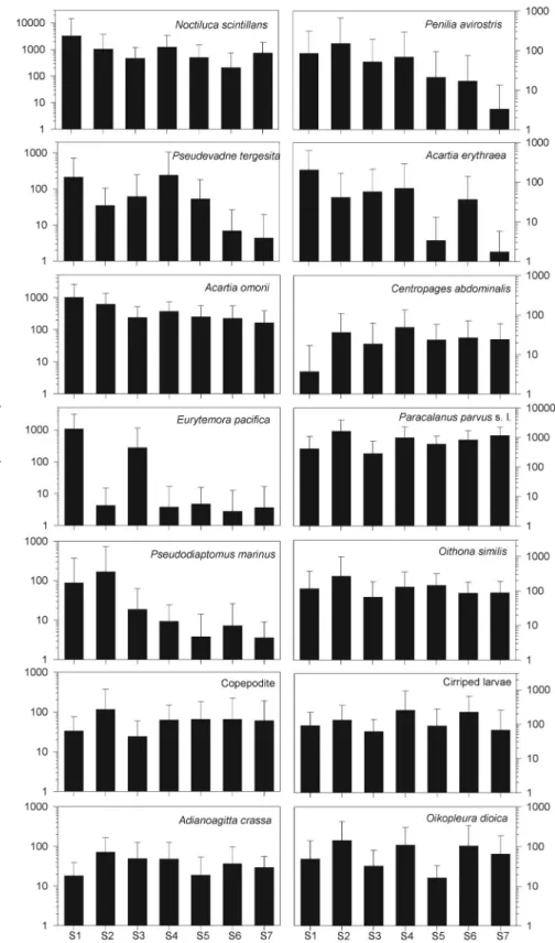
Spatial and temporal variations of zooplankton density, copepods density, diversity, and the most dominant taxon of zooplankton were significant (Table 3). Of the 3 domi- nant species, N. scintillans, A. omorii, and C. affinis showed the most significance between seasonal and spatial varia- tion. There were two groups based on spatial distribution:

those showing significantly higher density at inner region (e.g., N. scintillans, A. omorii, A. erythraea, E. pacifica, and P. marinus); those showing no significant spatial variation;

and those showing significantly low density in the outer regions (P. avirostris, P. tergestina, A. erythraea, E. pacifica, and P. marinus) (Fig. 4). The monthly variations in the density of dominant species showed that the most domi- nant species were generally highly abundant during June to October, corresponding to the period of high tempera-

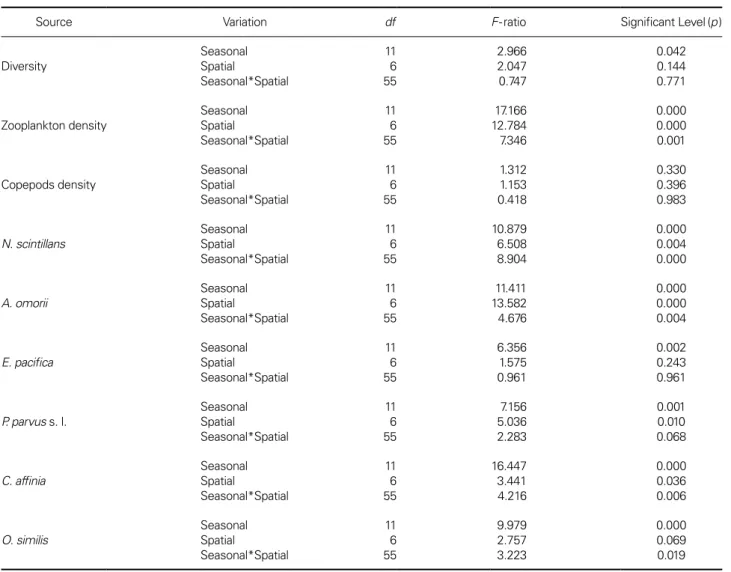
Table 3. Two-way analysis of variance

(ANOVA) summary results of the seasonal (12 months) and spatial (7 sampling stations) variations in the diversity and density of the dominant taxon of zooplankton in Gamak Bay

Source Variation df F-ratio Significant Level (p )

Diversity Seasonal

Spatial

Seasonal*Spatial

11 6 55

2.966 2.047 0.747

0.042 0.144 0.771

Zooplankton density Seasonal

Spatial

Seasonal*Spatial

11 6 55

17.166 12.784 7.346

0.000 0.000 0.001

Copepods density Seasonal

Spatial

Seasonal*Spatial

11 6 55

1.312 1.153 0.418

0.330 0.396 0.983

N. scintillans Seasonal

Spatial

Seasonal*Spatial

11 6 55

10.879 6.508 8.904

0.000 0.004 0.000

A. omorii

Seasonal Spatial

Seasonal*Spatial

11 6 55

11.411 13.582 4.676

0.000 0.000 0.004

E. pacifica Seasonal

Spatial

Seasonal*Spatial

11 6 55

6.356 1.575 0.961

0.002 0.243 0.961

P. parvus s. l. Seasonal

Spatial

Seasonal*Spatial

11 6 55

7.156 5.036 2.283

0.001 0.010 0.068

C. affinia Seasonal

Spatial

Seasonal*Spatial

11 6 55

16.447 3.441 4.216

0.000 0.036 0.006

O. similis Seasonal

Spatial

Seasonal*Spatial

11 6 55

9.979 2.757 3.223

0.000

0.069

0.019

Fig. 4. Spatial variation in the density of the dominant zooplankton taxa. Mean

(±SD) values of the density (ind. m

) data generated from 12 months of samples collected in Gamak Bay. The data are means with SD indicated by the error bars.

Abundance(ind. m-3 )

ture. However, their co-occurrence was different (Fig. 5).

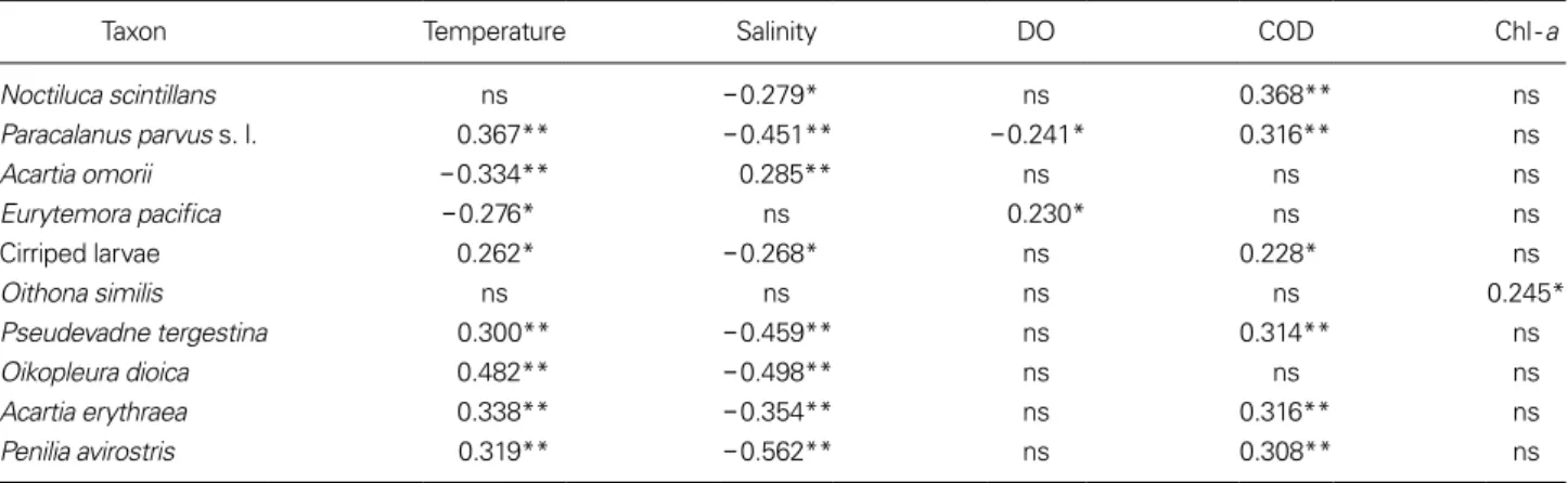
The results of Pearson’s correlation analysis showed some significant associations among the dominant taxa of zoo- plankton, temperature, salinity, DO, COD, and chl-a con- cen trations (Table 4). The density of N. scintillans cor- related positively with COD, but negatively with salinity;

whereas, the density of P. parvus s. l. correlated negatively with temperature and COD. The density of E. pacifica and A. omorii correlated negatively with temperature. On the other hand, the density of A. erythraea and Penilia avirostris correlated positively with temperature and COD, but nega- tively with salinity.

Zooplankton density showed no significant spatial varia- tion, having the highest mean density of (7,074±12,616) ind. m

at S1, and the lowest mean density of (1,908±

1,433) ind. m

at S3. There were two major spatial areas based on zooplankton density: a high-density area at inner region (S1 and S2), and a lower density area at central and outer regions (S4 to S7). However, the value of diversity in- dex showed significant spatial variations (F ⁼ 2.4, p ⁼ 0.04), with the highest mean diversity index at S5, and the lowest mean diversity index at S1. The numbers of species and den- sity did not show significant spatial variations (Fig. 6). How- ever, the number of species (F ⁼ 10.21, p < 0.001), den sity (F = 2.30, p = 0.018), and diversity (F = 3.60, p < 0.001) showed significant seasonal variations. Higher number of species and density were observed during June to Septem- ber excluding August, while higher diversity index was ob- served during August to October. There were two distinct regions based on all diversity indices used. The inner re- gion (S1 and S2) had significantly lower diversity than the central to outer regions.

3. Relationship of hydrographical factors in the zooplankton community

The influence of the hydrographic environment on the number of taxa, zooplankton density, diversity, and on the density of the three dominant species (N. scintillans, P.

parvus s. l., and A. omorii) were characterized using multi- ple regression analysis. Temperature, salinity, DO, COD, and chl-a concentrations were used as independent fac- tors in the multiple regression model to characterize their influence on the dependent variables of number of taxa, zooplankton density, diversity, and dominant species.

Significant multiple regression models were produced for the number of taxa (F ⁼ 16.67; adjusted R

⁼ 0.292;

p < 0.0001), zooplankton density (F = 14.12; adjusted R

⁼ 0.147; p < 0.0001), diversity (F ⁼ 6.11; adjusted R

= 0.186; p < 0.0001), N. scintillans (F = 12.29; adjusted R

⁼ 0.233; p < 0.0001), P. parvus s. l. (F ⁼ 18.51; adjusted R

= 0.184; p < 0.0001), and A. omorii (F = 24.33; adjusted R

⁼ 0.375; p < 0.0001) (Table 5). The model showed that temperature was the common predictor for diversity, and for N. scintillans and A. omorii of the dependent variables (P values were 0.008, 0.001, and 0.001 for diversity, N. scin- tillans, and A. omorii, respectively). For the number of taxa and zooplankton density, two additional variables of DO and salinity for the number of taxa (p < 0.05) and COD for zooplankton density (p < 0.05) were found as signifi- cant predictors (Table 5). Temperature was the significant common predictor variable for both N. scintillans (p < 0.05) and A. omorii (p < 0.05), and one additional variable of salinity (p < 0.05) was a significant predictor for P. parvus s.l. Multiple regression models with other species were not

Table 4. Pearson’s correlation coefficient between the monthly temperature, salinity, DO, COD, and chlorophyll-a

(chl-a) concentrations patterns and the monthly abundance of the dominant zooplankton species in Gamak Bay

Taxon Temperature Salinity DO COD Chl-a

Noctiluca scintillans ns -0.279* ns 0.368** ns

Paracalanus parvus s. l. 0.367** -0.451** -0.241* 0.316** ns

Acartia omorii -0.334** 0.285** ns ns ns

Eurytemora pacifica -0.276* ns 0.230* ns ns

Cirriped larvae 0.262* -0.268* ns 0.228* ns

Oithona similis ns ns ns ns 0.245*

Pseudevadne tergestina 0.300** -0.459** ns 0.314** ns

Oikopleura dioica 0.482** -0.498** ns ns ns

Acartia erythraea 0.338** -0.354** ns 0.316** ns

Penilia avirostris 0.319** -0.562** ns 0.308** ns

*p<0.05, **p<0.001, ns is not significant.

Fig. 5. Seasonal variation in the density of the dominant zooplankton taxa. Mean values of the density

(ind. m

) data generated from 12 months of samples collected in Gamak Bay.

Ln(abundance; ind. m-3 )

Table 5. Summary of the results of multiple regression analyses of the effects of environmental variables on the number of taxa, zooplank-

ton density, diversity, and the density of the three dominant species (N. scintillans, P. parvus s. l. and A. omorii )

Dependent variable Design summery (ANOVA) Independent variable Beta value Significant Level (p)

Number of taxa F = ^{16.67, R}

= ^0.292

p

0.0001 DO

Salinity −0.485

−1.818 0.000

Zooplankton density F = ^{14.12, R}

= ^0.147

p

0.0001 COD 0.996 0.000

Diversity F = ^{6.11, R}

= ^0.186 p

0.0001

Temperature COD DO

0.504 -0.380

0.528 0.008

N. scintillans F = ^{12.29, R}

= ^0.233

p

0.0001 DO

Temperature -8.530

- 3.312 0.000

P. parvus s. l. F = ^{18.51, R}

= ^0.184

p

0.0001 Salinity -14.964 0.000

A. omorii F = ^{24.33, R}

= ^0.375

p

0.0001 Temperature

DO 0.188

0.187 0.000

Fig. 6. Spatial and seasonal variations in the number of species, total zooplankton density, and diversity. The data are means with SD indi-

cated by the error bars.

Number of speciesAbundance(103

×

Spatial Temporal

Fig. 7. Temperature-Salinity-Density diagrams for dominant species of the zooplankton community. The density

(ind. m

) of the species was estimated by multiplying the numbers on the scale by 1 × ¹⁰

for each species.

Salinity(psu) Salinity(psu)

Temperature (°C)

significant, suggesting that the species were strongly influ- enced by the hydrographical variables.

In Gamak Bay, the five acartiid species (A. erythraea, A.

omorii, A. ohtsukai, A. pacifica, and A. sinjiensis) displayed distinct spatial and temporal distribution patterns. Of these, two showed seasonal fluctuation during the study period. Acartia omorii occurred from October to July when temperature ranged (4.8 to 24.8)°C (Fig. 7). The spatial and temporal variability of P. parvus s. l. in Gamak Bay was characterized as being continuous in the zooplankton throughout the year, showing a high peak in summer to au- tumn, but lowest in winter. High density of two cladocer- ans (Pseudevadne tergestina and Penilia avirostris) was found in July. It is possible that seasonal differences in the density and peaks in Gamak Bay are related to temperature and COD concentrations (Table 4).

The Temperature - Salinity - Density diagram showed differences in ecological requirements of the dominant species of zooplankton communities in Gamak Bay (Fig.

7). Noctiluca scintillans occurred intermittently throughout the year, as temperature and salinity of the regions again increased above 20°C and below 32 psu, respectively. The density of P. avirostris and P. tergestina peaked when tem- perature and salinity were 23°C and 29 psu, respectively.

In summer, A. erythraea showed high density when tem- perature and salinity ranged (22 to 28)°C, and from (30 to 32) psu, respectively, while A. omorii was most abundant at temperature of below 20°C and salinity of almost 33 psu.

Eurytemora pacifica is stagnant in eutrophic waters at the inner region. Its density is higher at temperature of below 10°C and salinity of almost 33 psu. Paracalanus parvus s.

l. was predominant in the whole bay area throughout the year. The density of P. parvus s. l. increased when the sa- linity decreased, and temperature ranged (10 to 25)°C.

Pseudodiaptomus marinus and O. similis had similar periods of density in the inner region. Their density was sharply decreased when temperature was below 23°C. Regarding occurrence, P. marinus showed high density at temperature of 23°C, and salinity of 29 psu. Small cyclopoid copepod O.

similis showed high density during warm seasons in Gamak Bay, when temperature and salinity were 20°C and 32 psu, respectively. Among zooplankton found in Gamak Bay, only Aidanosagitta crassa occurred during the study period.

Mass occurrences of A. crassa were observed in spring and autumn. High density of O. dioica was found when tem- perature and salinity ranged (17 to 24)°C, and (30 to 33) psu, respectively. The density of N. scintillans was also pos- itively correlated with COD concentration, indicating that

density of zooplankton might be largely influenced by high chl-a concentration.

DISCUSSION

Gamak Bay presented considerable spatial and temporal variability for hydrographic conditions and zooplankton community during the study period. Differences in the hy- drographic conditions and trophic status between the inner and outer regions of Gamak Bay were apparent. Zooplank- ton showed higher density at the inner region, but lower density at the outer region in Gamak Bay. Spatial and tem- poral variability of zooplankton by a few dominant species can sometimes occur in Gamak Bay under unstable situa- tions (Soh et al. 2002; Moon et al. 2006b). The zooplank- ton assemblages in Gamak Bay were dominated by N. scin- tillans (30.9%), P. parvus s. l. (24.3%), A. omorii (12.0%), E.

pacifica (5.7%), and cladocerans (4.1%). A similar domin- ance pattern by these same species also occurred in Gwang - yang Bay (Jang et al. 2004) and Jinhae Bay (Soh and Choi 2004). Noctiluca scintillans was found throughout the year, excluding September. It had high density when tempera- ture increased above 20°C, salinity decreased below 30 psu, and when chl-a was high while oxygen level was low. Nocti- luca scintillans contributed largely to the decrease of cope- pods at low salinity, because it was the only taxon exceed- ing the density of copepods in Gamak Bay (Soh et al. 2002;

Moon et al. 2006b). Increased density of N. scintillans may affect short-term variations of phytoplankton biomass thr- ou gh predation on eggs and copepods nauplii, thus influ- encing copepod populations (Sekiguchi and Kato 1976;

Kimor 1979; Daan 1987; Nakamura 1998). In Gamak Bay, diatoms were the most dominant phytoplankton group during June to September (Lee and Kim 2008). These re- sults support an association between the population of N.

scintillans and hydrographical factors, given their high spa- tial and temporal heterogeneity of zooplankton density in Gamak Bay.

The density of copepods was negatively impacted by

eutrophic condition in this study. Zooplankton communi-

ties with eutrophic condition appeared successively at inner

region, correlating well with the timing of autochthonous

species that dominated, such as E. pacifica and acartiid

species. Of these, E. pacifica was a predominant species at

the inner region during winter to early spring. This species

has long been considered as abundant in the zooplankton

community in Japanese Inlet waters (Ueda 1982; Uye et al.

2000) and the estuarine and coastal waters of Korea (Kim and Huh 1983; Kang et al. 1996; Soh et al. 2002; Moon et al.

2006b). Eurytemora species can produce resting eggs, which allows them to lie dormant in the sediment, and appear suddenly when conditions are favorable (Uye 1985; Ban and Minoda 1994; Viitasalo 1994). Most coastal copepods spend a portion of their life cycle in the sediment as resting eggs (Uye 1985; Marcus 1996). This might profoundly influence the dynamics of the zooplankton community (Hairston Jr et al. 2000). When the habitat environment is recovered, resting eggs are hatched. Our results support the notion that low temperature ( ^< 20°C) may be an import- ant cue to induce resting egg production of E. pacifica in Gamak Bay.

The spatial and temporal variability of five acartiids are similar to the thermal range for the occurrence of this spe- cies in the zooplankton found in previous work carried out in the central part of the Inland Sea of Japan (Liang and Uye 1996a), and the southern coasts of Korea (Park et al.

2001; Soh and Jeong 2003; Part et al. 2015). The seasonal variability of A. omorii is significantly correlated with tem- perature, probably resulting from its seasonal cycle and ecological requirement rules (Liang and Uye 1996a; Soh and Jeong 2003, Park et al. 2015). Temperature and salini- ty appear to provide A. erythraea a competitive advantage, allowing them to extend their distribution to the inner region during summer. Acartia erythraea is predominant in the shallow coastal waters of Korea during summer and autumn (Han et al. 1995; Kang et al. 1996; Soh and Choi 2004; Moon et al. 2006b) and the bottom in coastal waters during day, to maintain their position against weak wa- ter currents (Ueda et al. 1983). The spatial and temporal segregation and continued coexistence of Acartia species might be due to slight difference between species in terms of their adaptation abilities and preferences for certain hy- drographical conditions, such as temperature, salinity, and tidal exchange. These factors may play a key role in deter- mining their spatial and temporal distributions (Jeffries 1962; Ueda 1987; Soh and Jeong 2003; Moon et al. 2008;

Park et al. 2015). These results suggest that Gamak Bay is a preferred place with suitable temperature, salinity, and food for the five acartiids to control their populations.

Jang et al. (2004) investigated the seasonal distribution of P. parvus s. l. in Gwangyang Bay of Korea, which has a temperate domain similar to Gamak Bay. This species is one of the most dominant copepods in the estuarine and coastal habitat (Soh and Suh 1993; Han et al. 1995; Liang and Uye 1996b, Rong et al. 2002; Jang et al. 2004, 2015).

The occurrence pattern of Paracalanus sp. (as P. parvus s.

l.) in Fukuyama Harbor had a temperature range of (8.9 to 28.2)°C, with a high peak at temperature ranging (20.4 to 25.4)°C. The egg production rate of the natural population of P. parvus s. l. was constant. It did not show any district reduction until temperature warmed up to 25°C, showing acclimation to higher temperature (Liang and Uye 1996b).

Cladocerans can be the numerically dominant components of the zooplankton community in temperate, tropical, and subtropical regions (Clarke and Roff 1990; Kim and Onbé 1995). They are usually dominated by phytoplankton den- sity in coastal waters, especially cryptophytes in eutrophic Tolo Harbor in the eastern coastal waters of Hong Kong (Wong et al. 2006). According to Lee and Kim (2008), there is a high density of phytoplankton, such as diatoms, in June to September in Gamak Bay. This result indicates that they are favored by water stratification during summer, when small-sized phytoplankton dominates because of rel- atively high chl-a concentrations in the surface layer, which occurs in the inner region.

Temperature and salinity were the main hydrographi- cal factors regulating the spatial and temporal patterns of zooplankton in estuaries and coastal waters (Badylak and Phlips 2008; Sun et al. 2011; Park et al. 2015). In this study, the multiple regression for the association of hydrograph- ical factors with number of taxa, zooplankton density, di- versity, and dominant species differed, depending on the zooplankton community considered. In Gamak Bay, cope- pods (such as A. omorii , P. parvus s. l., and E. pacifica) and diversity co-varied with temperature (p < 0.05), salinity (p < 0.05), and DO concentration (p < 0.05), indicating a tight coupling between temperature and neritic copepods density, which had high values around the inner region (S1 to S3). Therefore, temperature is the most important variable that can describe the observed variability in diver- sity, and of N. scintillans, and A. omorii in Gamak Bay as a whole; and COD concentration is the additional variable for zooplankton density and diversity in the inner region.

Several studies that described spatial and temporal patterns of zooplankton density in Korean estuaries and coastal wa- ters considered the influence of both abiotic (e.g., tempera- ture and salinity) and biotic (phytoplankton and N. scintil- lans density) factors (Yoon and Choi 2002; Soh and Jeong 2003; Jang et al. 2004; Lee et al. 2006; Moon et al. 2006b;

Park et al. 2015). In Gamak Bay, seasonal temperature,

salinity, DO, and COD concentrations typically have im-

portant effects on the zooplankton community. Therefore,

these factors were considered in this study to determine

their possible impacts on the zooplankton community in Gamak Bay.

CONCLUSION

The present analysis showed that the seasonal cycle of zooplankton density and taxonomic composition was probably determined mainly by their preferences and tol- erances for specific temperature, salinity, chl-a, and COD concentrations. High nutrient input by freshwater dis- charge from near metropolitan city and Seomjin River into Gamak Bay resulted in significantly higher N. scintillans density, and also affected zooplankton density. The marked increase in the zooplankton density at the inner region during summer to autumn, when freshwater discharge was at its peak, suggested that the density was strongly relat- ed to temperature and freshwater inputs that could drive nutrient inputs, consequently affecting food supply in the system, due to intense continental drainage. Nevertheless, future studies that combine information on the density of N. scintillans and zooplankton and their daily consumption rates are needed, to quantitatively determine the extent to which predation influences the density and community structure of zooplankton in Gamak Bay.

ACKNOWLEDGEMENT

This research was supported by a grant from the National Institute of Fisheries Science (NIFS) of Korea (R2020029).

REFERENCES

Badylak S and EJ Phlips. 2008. Spatial and temporal distributions of zooplankton in Tampa Bay, Florida, including observations during a HAB event. J. Plankton Res. 30:449-465.

Ban S and T Minoda. 1994. Induction of diapause egg production in Eurytemora affinis by their own metabolites. Hydrobiolo- gia 292/293:185-189.

Cembella AD, DA Ibarra, J Diogene and E Dahl. 2005. Harmful algal blooms and their assessment in Fjorda and coastal em- bayments. Oceanography 18:158-171.

Chisholm LA and JC Roff. 1990. Abundance, growth rates, and production of tropical neritic copepods off Kingston Jamaica.

Mar. Biol. 106:79-89.

Cho EI, CI Chung and SM Lee. 1996. Estimation of carrying capacity in Kamak Bay. II. estimation of carrying capacity of

oyster culture ground. J. Korean Fish. Soc. 29:709-715.

Clarke C and JC Roff. 1990. Abundance and biomass of herbiv- orous zooplankton off Kingston, Jamaica, with estimates of their annual production. Estuar. Coast. Shelf Sci. 31:423-437.

Clarke KR and RM Warwick. 2001. Change in Marine Communi- ties: an Approach to Statistical Analysis and Interpretation, 2

Edn., PRIMER-E, Limited, Phymouth Marine Laboratory, United Kingdom.

David V, B Sautour, R Galois and P Chaddy. 2006. The paradox high zooplankton biomass-low vegetal particulate organic matter in high turbidity zones: what way for energy transfer?

J. Exp. Mar. Biol. Ecol. 333:202-218.

Hairston Jr NG, AM Hansen and WR Schaffiner. 2000. The effect of diapause emergence on the seasonal dynamics of a zoo- plankton assemblage. Freshw. Biol. 45:133-145.

Han DH, SY Hong and CW Ma. 1995. Distribution of zooplankton in Deukryang Bay. J. Korean Fish. Soc. 28:517-532.

Jang MC, KS Shin, PG Jang, WJ Lee and KH Choi. 2015. Meso- zooplankton community in a seasonally hypoxic and highly eutrophic bay. Mar. Freshw. Res. 66:719-729.

Jang MC, PG Jang, KS Shin, DW Park and M Chang. 2004.

Seasonal variation of zooplankton community in Gwangyang Bay. Korean J. Environ. Biol. 22:11-29.

Kang HS, MH Seo, YS Yang, EO Park, YH Yoon, D Kim, HG Jeong and HY Soh. 2018. Zooplankton and neustonic microplastics in the surface layer of Yeosu coastal areas. Korean J. Environ.

Biol. 36:11-20.

Kang YS, JS Park, SS Lee, HG Kim and PY Lee. 1996. Zooplank- ton community and distributions of copepods in relation to eutrophic evaluation in Chinhae Bay. J. Korean Fish. Soc.

29:415-430.

Kim DY and HT Huh. 1983. Seasonal variations of copepods in Garolim Bay. Bull. Kor. Ocean. Res. Dev. Ins. 5:29-35.

Kim JB, SY Lee, J Yu, YH Choi, CS Jung and PY Lee. 2006. The characteristics of oxygen deficient water mass in Gamak Bay. J. Kor. Soc. Mar. Environ. Eng. 9:216-224.

Kim SW and T Onbé. 1995. Distribution and zoogeography of the marine cladoceran Penilia avirostris in the northwestern Pacific. Bull. Plankton Soc. Japan 42:19-28.

Kimmel DG and M Romen. 2004. Long-term trends in mesozo- oplankton abundance in Chesapeake Bay, USA: influence of freshwater input. Mar. Ecol. Prog. Ser. 267:71-83.

Kimor B. 1979. Predation by Noctiluca miliaris Souriray on Acartia tonsa Dana eggs in the inshore waters of southern Califor- nia. Limnol. Oceanogr. 24:568-572.

Leandro SM, F Morgado, F Pereira and H Queiroga. 2007. Tem-

poral changes of abundance, biomass and production of

copepod community in a shllow temperate estuary (Ria de

Aveiro, Portugal). Estuar. Coast. Shelf Sci. 74:215-222.

Lee CR, C Park, SR Yang and YS Sin. 2006. Spatio-temporal vari- ation of mesozooplankton in Asan Bay. The Sea 11:1-10.

Lee KH and KD Cho. 1990. Distribution of the temperature and salinity in Kamak Bay. Bull. Korean Fish. Soc. 23:25-39.

Lee MO and JK Kim. 2008. Characteristics of algal blooms in the southern coastal waters of Korea. Mar. Environ. Res.

65:128-147.

Lee YS and SY Moon. 2006. The water quality in the soho coastal seawaters of Gamak Bay before and after a typhoon. The Sea 11:117-123.

Liang D and S Uye. 1996a. Population dynamics and production of the planktonic copepods in a eutrophic inlet of the Inland Sea of Japan. II. Acartia omorii. Mar. Biol. 125:109-117.

Liang D and S Uye. 1996b. Population dynamics and production of the planktonic copepods in a eutrophic inlet of the Inland Sea of Japan. III. Paracalanus sp. Mar. Biol. 127:219-227.

Marcus NH. 1996. Ecological and evolutionary significance of resting eggs in marine copepods: past, present, and future studies. Hydrobiologia 320:141-152.

Moon SY, HJ Oh and SY Kim. 2009. Short-term variations of me- sozooplankton related to the environmental factors in Gamak Bay during summer, 2006. J. Environ. Sci. 18:21-32.

Moon SY, HY Soh, SD Choi, CS Jung, SY Kim and YS Lee. 2006a.

Effect a low-oxygen layer on the vertical distribution of zoo- plankton in Gamak Bay. Korean J. Environ. Biol. 24:240-247.

Moon SY, HS Yoon, HY Soh and SD Choi. 2006b. Environmental factors and variation characteristics of zooplankton communi- ties in Gamak Bay. Ocean Polar Res. 28:79-94.

Nakamura Y. 1998. Biomass, feeding and production of Noctiluca scintillans in the Seto Inland Sea, Japan. J. Plankton Res.

20:2213-2222.

Odum HT. 1983. Systems Ecology: An Introduction. John Wiley and Sons Inc, New York.

Park EO, HL Suh and HY Soh. 2015. Spatio-temporal distribution of Acartia (Copepoda: Calanoida) species along a salinity gra- dient in the Seomjin River estuary, South Korea. J. Nat. Hist.

49:1-14.

Park YC and KS Choi. 2002. Growth and carrying capacity of pa- cific oyster, Crassostrea gigas in Kamak Bay, Korea. Korean J.

Environ. Biol. 20:378-385.

Parsons TR, Y Maita and CM Lalli. 1984. A Manual of Chemical and Biological Methods for Seawater Analysis. Pergamon Press, New York. p. 173.

Ramfos A, S Isari, S Somarakis, D Georgopoulos, C Koutsikopou- los and N Fragopoulu. 2006. Mesozooplankton community structure in offshore and coastal waters of the Ionian Sea (eastern Mediterranean) during mixed and stratified condi- tions. Mar. Biol. 150:29-44.

Roman M, X Zhang, C McGilliard and W Boicourt. 2005. Sea- sonal and annual variability in spatial patterns and plankton biomass in Chesapeake Bay. Limnol. Oceanogr. 50:480-492.

Romen MR, AL Guazens, WK Rhinehart and JR White. 1993.

Effects of low-oxygen waters on Chesapeake Bay zooplank- ton. Limnol. Ocenogr. 38:1603-1614.

Rong W, H Zhang, K Wang and T Zuo. 2002. Distribution and population dynamics of Paracalanus parvus, Paracalanus crassirostris, and Acartia bifilosa (Copepoda, Calanoida) in the Bohai Sea. Chin. J. Oceanol. Limnol. 20:348-357.

Sekiguchi H and T Kato. 1976. Influence of Noctiluca’s predation on the Acartia population in Ise Bay, Central Japan. J. Ocean- ogr. 32:195-198.

Seo JY, SH Park, JH Lee and JW Choi. 2012. Structural changes in macrozoobenthic communities due to summer hypoxia in Gamak Bay, Korea. Ocean Sci. J. 47:27-40.

Shannon E and W Weaver. 1963. The Mathematical Theory of Communication. Illinoise Univ. Press, Urbana, IL.

Shim JH and I Ro. 1982. The composition and abundance distri- bution of zooplankton in the vicinity of Yeosu, Korea. Proc.

Coll. Nat’l. Sci. Seoul Nat’l. Univ. 7:165-183.

Siokou-Frangou I and E Papathanassiou. 1991. Differentiation of zooplankton populations in a polluted area. Mar. Ecol. Prog.

Ser. 76:41-51.

Soh HY and HL Suh. 1993. Seasonal fluctuation of the abun- dance of the planktonic copepods in Kwangyang Bay. Korean J. Environ. Biol. 11:26-34.

Soh HY, IT Lee, YH Yoon, SD Choi, SN Lee, MI Han, BS Kim, YH Kang and WB Lee. 2002. Species composition and occur- rence patterns of zooplankton in Gamag Bay. Korean J. Envi- ron. Biol. 20:118-129.

Soh HY and SD Choi. 2004. Species composition and occur- rence patterns of zooplankton in Jinhae Bay. Korean J. Envi- ron. Biol. 22:43-56.

Sun XH, S Sun, CL Li and GT Zhang. 2011. Seasonal and spatial variability in egg production, abundance and production of small copepods in and near Jiaozhou Bay, China. J. Plankton Res. 33:741-750.

The Oceanographic Society of Japan. 1980. A Guide to Ocean- ographic Observations. The Oceanogaphy Society of Japan, Tokyo. p. 428.

Ueda H. 1982. Zooplankton investigations in Shijiki Bay II. Zoo- plankton communities from September 1975 to April 1976, with special reference to distributional characteristics of inlet copepod. Bull. Seikai. Reg. Fish. Res. Lab. 58:1-22.

Ueda H. 1987. Temporal and spatial distribution of the two closely

related Acartia species A. omorii and A. hudsonica (Copepo-

da, Calanoida) in a small inlet water of Japan. Estuar. Coast.

Shelf Sci. 24:691-700.

Ueda H, A Kuwahara, M Tanaka and M Azeta. 1983. Underwater observations on copepod swarms in temperate and subtrop- ical waters. Mar. Ecol. Prog. Ser. 11:165-171.

Uriarte I and F Villate. 2004. Effects of pollution on zooplankton abundance and distribution in two estuaries of the Basque coast (Bay of Biscay). Mar. Pollut. Bull. 49:220-228.

Uye S. 1985. Resting egg production as a life history strategy of marine planktonic copepods. Bull. Mar. Sci. 37:440-449.

Uye S, T Shimazu, M Yamamuro, Y Ishitobi and H Kamiya. 2000.

Geographical and seasonal variations in mesozooplankton abundance and biomass in relation to environmental pa- rameters in Lake Shinji-Ohashi River-Lake Nakaumi brack- ish-water system, Japan. J. Mar. Syst. 26:193-207.

Valiela I. 1991. Ecology of coastal ecosystems. pp. 57-76. In:

Fundamentals of Aquatic Ecology (RSK Barnes and KH Mann, 2nd eds.). Oxford: Blackwell Scientific, Oxford, UK.

Viitasalo M and T Katajisto. 1994. Mesozooplankton resting eggs in the Baltic Sea: identification and vertical distribution in lam- inated and mixed sediments. Mar. Biol .120:455-466.

Winkler G, JJ Dodson, N Bertrand, D Thivierge and WF Vincent.

2003. Trophic coupling across the St. Lawrence River estua- rine transition zone. Mar. Ecol. Prog. Ser. 251:59-73.

Wong CK, XJ Liu, YY Siu and JS Hwang. 2006. Study of selective feeding in the marine cladoceran Penilia avirostris by HPLC pigment analysis. J. Exp. Mar. Biol. Ecol. 331:21-32.

Zar JH. 1984. Biostatistical Analysis. Prentice Hall Inc., Engle-

wood Cliffs, NJ.