풍력에너지저널 pp. 36~44
5 MW 풍력 터빈 최적 제어 설계 평가1)
이자스리칸트레디*․황정현**․허성호***
Evaluation of Optimal Control Designs for a 5 MW Wind Turbine
Yiza Srikanth Reddy*, Jeong-Hyeon Hwang** and Sung-Ho Hur***
Key Words : Wind turbine control (풍력터빈제어), Linear quadratic Gaussian (선형 가우시안), Model predictive control (모델예측제어), Proportional-Integral-Differential controller (비례적분미분 제어기)
ABSTRACT
Optimal controllers are designed for a 5 MW variable-speed horizontal-axis wind turbine using Model Predictive Control (MPC) and Linear Quadratic Gaussian (LQG) control. The control design models required as part of the optimal control design are obtained using a high-fidelity aeroelastic model (i.e., DNV-GL Bladed).
The optimal controllers are subsequently designed based on these control design models linearised in three operating regions: below rated (region 1), just below rated (region 2), and above rated (region 3) wind speeds.
Various different simulation results are presented to demonstrate that the optimal controllers yield improved results compared to the conventional PID controller in terms of dealing with the drive-train mode; that is, while the standard PID controller requires a drive-train damper, optimal controllers, especially MPC, do not require such a damper to remove oscillation in the drive-train mode. Finally, a comparison between the two optimal controllers demonstrates that overall, MPC outperforms LQG controllers.
1. INTRODUCTION
In recent years, wind energy has become one of
* School of Electronic and Electrical Engineering, Kyungpook National University, PhD student
** School of Electronic and Electrical Engineering, Kyungpook National University, Msc student
*** School of Electronics Engineering, Kyungpook National University, Professor (Corresponding Author)
E-mail : [email protected]
DOI : https://www.doi.org/10.33519/kwea.2021.12.1.005 Received : December 23, 2020, Revised : February 9, 2021, Accepted : February 9, 2021
the most economical renewable energy sources due to its free and infinitely available nature with no harmful waste products. A wind turbine converts the kinetic energy from the wind into mechanical energy. It is then converted into electricity, which is subsequently transmitted to the power grid. The rotor and nacelle are the key components in the wind turbine and play a significant role in energy conversion [1,2]. Fig. 1 depicts a simplified schematic diagram of a wind turbine. When wind blows towards the blades, the hub rotates due to aerodynamic force, which is transmitted through drive-train consisting of a gearbox, which is responsible for increasing generator speed.
Fig. 1 Main components of a horizontal-axis variable- speed wind turbine
In this paper, we evaluate two optimal controller designs as opposed to the existing standard PID controller for a 5 MW variable-speed horizontal axis wind turbine having three blades.
The outline of control of a variable speed wind turbine could be classified into two parts-the determination of the operating strategy and its synthesis [3,4]. The control synthesis is concerned with designing single input single output linear controllers in different operating regions, while control strategy involves smoothly combining these controllers. This paper is only concerned with control synthesis.
In this paper, model predictive control (MPC) [5,6]
and linear quadratic Gaussian (LQG) [7,8] control are considered. Other control methods such as H∞
[9] could also be equally significant. The overall control design steps in operation and pursed in this study can be briefly summarised as follows:
(1) Development of linear control design models in each operating regions, followed by model reduction.
(2) Design of control synthesis based on the design models from (1) in each operating region.
Linear models of the Supergen Wind Energy Consortium (Supergen) 5 MW exemplar turbine at 8 (region 1), 10 (region 2), and 16 (region 3) m/s are attained in the state space form using DNV-GL
Bladed software using its in-built linearisation toolbox. These linear models are too complex and thus are significantly reduced using an order reduction method. Based on these linear models MPC and LQG controllers are developed and their performance compared.
The wind speed model and linear models obtained using Bladed are reported in Section 2. This is followed by the order reduction of the linear models.
Brief descriptions of MPC and LQG controllers are included in Section 3 and Section 4, respectively. In Section 5, simulation results are demonstrated in comparison to each other, which is followed by conclusions in Section 6. The standard PID controller requires a drive-train damper [10].
Simulation results are presented to show that the drive-train damper is not required when MPC controller is used, in comparison to the PID and LQG controllers. On the other hand, LQG also does not require a drive-train damper in regions 1 and 2 only, which is a significant advantage.
2. WIND SPEED AND LINEAR MODEL
2.1. Wind speed model
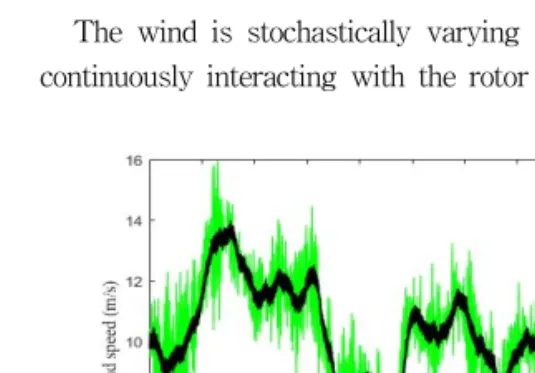
The wind is stochastically varying with time and continuously interacting with the rotor [2].
Fig. 2 Effective wind speed with rotational sampling (green) vs point wind speed (black) at a mean wind speed of 10 m/s
The effective wind speed is wind speed averaged over the rotor area such that the spectrum of aerodynamic torque remains unchanged. It can be obtained by filtering the point wind speed.
The effective wind speed is processed once more to incorporate the effect of rotational sampling [11].
Point wind speed and effective wind speed with rotational sampling used here are shown in Fig. 2.
2.2. Wind turbine linear model
A dynamic model is linearised from the Bladed model of the Supergen 5 MW exemplar turbine for three different operating regions, below rated wind speed (8 m/s), just below rated wind speed (10 m/s), and above rated wind speed (16 m/s). In the state space realisation, they have the following form:
∆xt A∆xt B∆uTt
∆yt C∆xt D∆uTt
(1)
where A, B, C, D denote the state space matrices.
∆ yt Rn, ∆ uTt Rm and ∆xt Rp (where n and m are respectively 2 and 3 at each mean wind speed, and p is 240) are defined as
∆yt yt yopt
∆uTt uTt uopt
∆xt xt xopt
(2)
where yt , uTt, and xt represent the output, input and states, respectively, and yopt uopt
andxopt are the operating points around which the models are linearised. A resulting Matlab/
SIMULINK simulation model is illustrated in Fig. 3.
The outputs for the for the linear models are (1) Measured generator speed
(2) Nacelle fore-aft acceleration
The inputs for the for the linear models are (1) Wind speed
(2) Pitch angle (3) Generator torque
Fig. 3 Bladed linearised wind turbine model
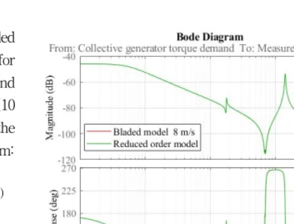
Fig. 4 Frequency response of Bladed model and reduced order model at a mean wind speed of 8 m/s
Fig. 5 Frequency response of Bladed model and reduced order model at a mean wind speed of 10 m/s
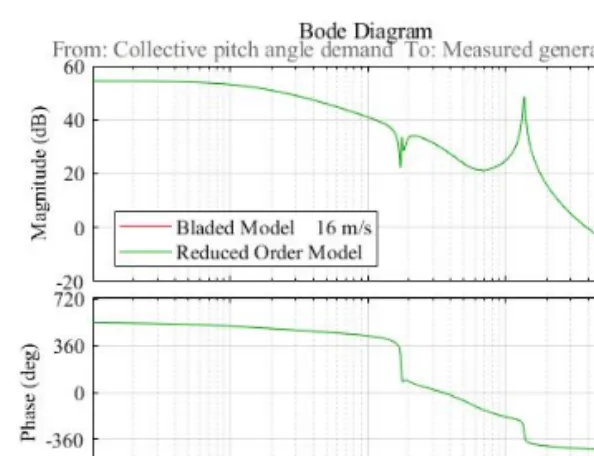
Fig. 6 Frequency response of Bladed model and reduced order model at a mean wind speed of 16 m/s As mentioned earlier, the linearised models contain 240 states making the realisation and tuning of MPC and LQG controllers highly sophisticated.
Thus, to design MPC and LQG controllers, the models need to be reduced. By using Match-DC-Gain model reduction algorithm [12], which is used to eliminate the weakly coupled states (states with smallest Hankel singular values); that is, the Match-DC-Gain method alters the remaining states to preserve the DC gain.
The open loop frequency responses of the original models, containing 240 states for 8, 10, and 16 m/s are depicted in Fig. 4, 5, and 6, respectively, in comparison to the frequency response of the reduced order models, which contain 20 states only. The results demonstrate that the original model and the reduced model exhibit almost identical characteristics within the meaningful frequency range.
When a controller is designed at below rated wind speed and just below rated wind speed, wind speed is considered to be disturbance, dtR, and the pitch angle is set to zero modifying (1) as follows:
∆xt A∆xt Bu∆u t Bd∆dt
∆yt C∆xt Du∆u t Dd∆dt
(3)
where yt R, utR, and xtR represent the generator speed, generator torque, and states, respectively.
Likewise when designing controllers at above rated wind speed, pitch angle becomes the only input while wind speed is consider to be disturbance, dtR, and the generator torque is set to zero modifying (1) as follows:
∆xt A∆xt Bu∆u t Bd∆dt
∆yt C∆xt Du∆u t Dd∆dt
(4)
where yt R, utR, and xtR represent the generator speed, pitch angle, and states, respectively.
Therefore, MPC and LQG controllers as the control design model deploy the following single input, single output equations:
∆xt A∆xt Bu∆u t
∆ygt C∆xt Dug∆u t
(5)
where ygt R denotes generator speed and Dug
is zero since MPC does not allow direct feedthrough.
3. MODEL PREDICTIVE CONTROL
MPC is revised in this section. It is a multivariable control algorithm consisting of an internal dynamic model of the plant, as reported in Section 2, a cost function over the prediction horizon, and an optimisation algorithm minimising the cost function, which is a function of the control input u.
3.1. Controller description
MPC can be designed based on the following state space model, which can be derived by discretising the continuous model in (5).
xk Axk Buuk yk Cgxk
(6)
where A Bu and denote the state space matrices. yk xk and represent the output, input and states, respectively. The prediction equation for MPC can be derived as follows [13] (note that D is 0 since no direct feed through is allowed in MPC)
xk
xk
⋮ xk p
A A
⋮ Ap
xk
Bu ⋯
ABu Bu ⋯
⋮ Ap Bu
⋮ Ap Bu ⋮
Ap B
⋮
⋯
uk
uk
⋮ uk p X
→ Pxx Hxx u
→
(7)
yk
yk
⋮ yk p
CgA CgA
⋮ CgAp
xk
CgBu ⋯
CgABu CgBu ⋯
⋮ CgAp Bu
⋮ CgAp Bu
⋮ CgAp B ⋮
⋯ u
→ y
→ P H
(8)
where Pxx, Hxx, P, H denote the prediction state space matrices and X
→, y
→, and u
→ represent the prediction states, outputs, and inputs respectively. p denotes prediction horizon and u
→ can be rewritten as
uk
uk
⋮ uk c uk c
⋮ uk c
u
→
(9)
where c represents control horizon.
The control input is calculated by minimising the following cost function [14]:
J ║r Hu Pxk Ld║ ║u║ (10) subject to the following constraints
u
i≤ ui≤ ui (11)
∆ui≤ ∆ui≤ ∆ui (12)
where ui represents the upper limit on ui,
ui the lower limit, and r the reference signal. H and P denote the prediction state space matrices. L is a vector of ones whose size is dependent on prediction horizon, and ∆ui the rate of change of input.
The first term in the cost function is related to the reference tracking error and d is included to give unbiased predictions and offset corrections. The second term in optimisation function is to reduce the control effort. Hence, gives a trade of between these two conflicting problems. xk denotes measured states at each time step, which come from internal model of the plant.
The procedure for implementation of MPC controller can be summarised as follows:
(1) At each time step, the current plant states are measured and the control sequence is calculated by solving the cost function over the prediction horizon in the future.
(2) The first value is only applied to the system and the remaining values are discarded. Then the plant states are sampled and the optimisation function is recalculated starting from the new current state.
(3) The prediction horizon keeps being shifted forward and for this reason MPC is also called receding horizon control.
4. LINEAR QUADRATIC GAUSSIAN CONTROL
Linear quadratic Gaussian control is a combination of Kalman filter and a linear quadratic regulator (LQR) [15,16]. Kalman filter estimates the states and LQR controls the plant using these state estimates from Kalman filter. In general, the system consists of process noise and measurement noise. LQG control gives the optimal control input to the plant
by minimising the effect of measurement and process noise. LQG is briefly summarised in this section.
4.1. Kalman filter
In general, a system is corrupted by process noise and measurement noise, with additional noise terms as follows:
xt Axt Buu t wt
ygt Cgxt Dugu t vt
(13)
where A, Bu, Cg, Dug denote the state space matrices and ygt, ut , x t , w t , vt
represent the output (generator speed), input (torque or pitch angle), states, white process noise, and measurement noise respectively. The following assumptions could be made:
Ewt Evt (14)
EwtwTt QN (15)
EvtvTt RN (16)
EwtvTt NN (17)
where QN, RN, and NN represent the process noise covariance matrix, measurement noise covariance matrix, and cross-covariance matrix respectively.
The state estimates, xt, that minimise the following steady-state error covariance can be written as [17]
P lim
t→∞
Ext xTtxt xTt (18) where x t and xt denote the states and states estimation respectively.
The optimal solution is the Kalman filter with the following equation:
xt Axt Bu t Kyt yt (19)
The estimator makes use of the inputs, u(t), and the measured output, y(t), to generate the output estimates, yt , and state estimates, xt.
The Kalman filter gain, K, is derived by solving the following algebraic Riccati equation [18].
K PCT BdQNDT NN ⋯
RN DdNN NNTDdTQNDdT
(20)
4.2 Linear quadratic regulator
LQR solves the optimisation problem offline:
J ║xTtQ x t║ ║uTtR u t║ (21) where Q is an r × r symmetric positive semi-definite matrix and R an m × m symmetric positive-definite matrix. The first part in the optimisation problem is to reduce the reference tracking error and the second part is to reduce the control effort.
The optimal state-feedback LQR controller for minimising the performance index, J, in (21) is a simple matrix gain of the following form:
u t L xt (22)
where xt is the state estimates from the Kalman filter, and L is a m × n matrix as follows:
L DuTQ Du R BTP DuTQ C (23) P is the unique positive-definite solution to the following algebraic Riccati equation:
ATP P A CTQ C P B CTQ Du ⋯
DuTQ Du R BTP DuTQ C
(24)
5. RESULTS
The measured output at each mean wind speed (i.e. generator speed) is illustrated in Fig. 7. The time responses for the MPC and LQG based controllers at mean wind speeds of 10 and 16 m/s are satisfactory in terms of fluctuations as they remains well below 12 %, which are normally within the controller design specification.
Fig. 7 MPC and LQG based on Bladed linearised model;
generator speed (control output); time response for a mean wind speed of 8 m/s, 10 m/s, and 16 m/s.
Fig. 8 MPC and LQG based on Bladed linearised model;
torque demand (8 and 10 m/s) and pitch angle demand (16 m/s) (control input); time response for a mean wind speed of 8 m/s, 10 m/s, and 16 m/s.
The corresponding control inputs, i.e., torque and pitch angle demand are also depicted in Fig. 8. As stated earlier, the turbine operates in region 1 at 8 m/s, in region 2 at 10 m/s, and in region 3 at 16 m/s. Generator speed is controlled by adjusting torque in regions 1 and 2 by pitching in region 3.
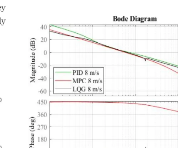
Fig. 9 MPC and LQG based on Bladed linearised model for a mean wind speed of 8 m/s; open loop frequency response; Ts=0.02 s (sampling time) for MPC.
The corresponding open-loop frequency responses are shown in Fig. 9, 10, and 11. The open-loop system is referred to as the product of the process (i.e. the turbine model) and the controller (open loop). The controllers should be tuned to give a gain crossover frequency in the range of 0.6 to 2 rad/s [19], due to the characteristics of wind. Gain crossover frequencies over this range may could lead to too aggressive, leading to actuator saturation, especially in higher wind speeds. Gain crossover frequencies below this range could lead to too slow control action.
At a mean wind speed of 8 m/s, Fig. 9 depicts that the gain crossover frequencies of the PID, MPC, and LQG controllers are approximately in the satisfactory range of 0.6 to 2 rad/s, and also there is no peak above 0 dB. It implies that these controllers are neither too aggressive nor too slow, and they all produce satisfactory results.
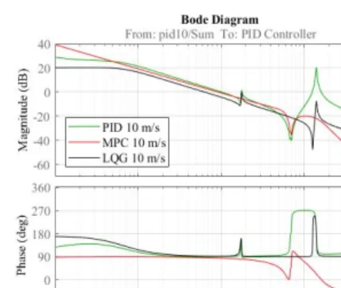
Fig. 10 MPC and LQG based on Bladed linearised model for a mean wind speed of 10 m/s;
open loop frequency response; Ts=0.02 s (sampling time) for MPC.
Fig. 11 MPC and LQG based on Bladed linearised model for a mean wind speed of 16 m/s; open loop frequency response;
Ts=0.1 s (samplimg time) for MPC.
It shows that these controllers are neither too aggressive nor too slow. However, the peak at around 14.15 rad/s – which is the drive-train mode - from the PID controller remains mostly above 0 dB at higher frequencies for mean wind speed of 10 m/s, indicating that the controller would be sensitive to uncertainty and noise. The peaks are normally removed by applying a drive-train damper [10]; that is, the PID controller requires a drive-train damper to keep the peak at around 14.15 rad/s below 0 dB.
However, it is very important to highlight that the MPC and LQG controllers keep the peak below 0
dB without a damper as shown in Fig. 10.
Only for mean wind speed of 16 m/s, the MPC based controller is more sensitive to sampling time, Ts, and 0.1 s needs to be chosen to improve the results. Fig. 11 illustrates that the gain crossover frequencies are also approximately in the range of 0.6 to 2 rad/s for these controllers. It demonstrates that these controllers are neither too aggressive nor too slow. However, the peak from the PID and LQG controllers remain mostly above 0 dB at around 13.83 rad/s, indicating that the PID and LQG controllers would be sensitive to uncertainty and noise.
Finally although the time response of the LQG based controller for 16 m/s seems satisfactory as depicted in Fig. 7, the high frequency oscillation observed at around 13.83 rad/s for 16 m/s in Fig. 11 would result in increased loads on the rotor that would propagate down the drive-train and impact the drive-train components, such as shaft, gearbox.
Hence, the overall LQG design at 16 m/s is not satisfactory.
6. CONCLUSIONS
Linear dynamic models of the Supergen 5 MW exemplar wind turbine are constructed for three operating regions, below rated wind speed (8 m/s), just below rated wind speed (10 m/s), and above rated wind speed (16 m/s).
This paper demonstrates the design of different controllers; that is, MPC and LQG, in comparison to each other as well as the more standard PID controllers. The time responses for the MPC and LQG based controllers at mean wind speeds of 10 and 16 m/s are satisfactory in terms of fluctuations as they remains well below 12 %, which are normally within the controller design specification.
Open loop frequency responses illustrate that both the optimal controllers (MPC and LQG) outperform the PID controllers in regions 1 and 2, and only the MPC controller outperforms the PID controller in
region 3. This is mainly because the MPC optimal controllers are able to remove the drive-train peak without having to incorporate a damper in contrast to the PID controllers.
Finally, the optimal controllers, especially the LQG controllers, can be more difficult and time- consuming to tune than the PID controller.
7. ACKNOWLEDGEMENT
This work was supported by Korea Institute of Energy Technology Evaluation and Planning (KETEP) grant funded by the Korea government (MOTIE)(20203020020020, Feasibility Study on 40years Life Wind Turbine)
8. REFERENCES
[1] Luo N, Vidal Y, and Acho L., 2014, Wind tur- bine control and Monitoring, Springer: Cham (ZM), Switzerland.
[2] Burton, T., Jenkins, N., Sharpe, D., and Bossanyi E., 2001, Wind Energy Handbook, John Willey &
Sons, Ltd.: Chichester, UK.
[3] Leithead WE and Connor B, 2000, Control of variable speed wind turbines: design task, inter- national journal of control, p. 1189-1212.
[4] Garcia-Sanz M and Houpis CH, 2012, Wind en- ergy Systems: Control Engineering Design, CRC Press: Boca Raton, Florda, USA.
[5] Camacho EF and Bordons C, 2011, Model Predictive Control in the Process Industry (Advances in Industrial Control), Springer:
London, UK.
[6] Grancharova AI and ohnsen TA, 2012, Explicit Nonlinear Model Predictive Control: Theory and applications, Springer-verlag: Berlin hei- delberg, Berlin.
[7] Grimble MJ and Johnson TA, 1988, Optimal con- trol and Stochastic Estimation: Theory and Applications, Wiley: New York, USA.
[8] Trenteleman H, Stoorvoged AA, and Hautus M, 2012, Control theory for Linear Systems (Communications and control Engineering), Springer: London, UK.
[9] Skogestad S and Postlethwaite, 2005, Multivariable Feedback Control: Analysis and design (2nd edn), Wiley.
[10] Chatzopoulos A, 2011, Full envelope wind tur- bine controller design for power regulation and tower load reduction, Ph.D. Thesis, The uni- versity of Strathclyde.
[11] Leithead WE, 1992, Effective wind speed models for simple wind turbine simulations, Proceedings of 14th British Wind Energy Association (BWEA) Conference, Nottingham, pp.321-326.
[12] Varga A, 1991, Balancing-Free Square-Root Algorithm for Computing Singular Perturbation Approximations, Proc. of 30th IEEE CDC, Brighton, pp. 1062-1065.
[13] Rossiter JA, 2005, Model-based Predictive Control: A Practical Approach, CRC Press, Boca Raton, Florida.
[14] Maciejowski JM, 2000, Predictive control with constraints, Prentice Hall: New York, USA.
[15] Clements DJ and Anderson BDO, 1978, Singular Optimal Control: The Linear-Quadratic Problem, Springer-Verlag, London.
[16] Hespanha JP, Undergraduate Lecture Notes on LQG/LQR Controller Design, University of California Snata Barbara, Electrical and Computer Engineering.
[17] Franklin GF, Powell JD, and Workman WL 1990, Digital Control of Dynamic Systems (Second), Addison-Wesley, HalfMoon Bay, USA.
[18] Lewis F, 1986, Optimal Estimation, John Wiley
&Sons, Inc, Hoboken.
[19] Leith DJ and Leithead WE, 1996, Appropriate realization of gain-scheduled controllers with application to wind turbine regulation, International journal of control, Vol. 65, No, 2, PP. 223-248.