Multivariate Process Capability Indices for Skewed Populations with Weighted Standard Deviations

(1)

가중표준편차를 이용한 비대칭 모집단에 대한 다변량 공정능력지수

장영순

¹

․배도선

^2†

1

LG CNS 컨설팅 부문 /

²

한국과학기술원 산업공학과

Multivariate Process Capability Indices for Skewed Populations with Weighted Standard Deviations

Young Soon Chang

¹

․Do Sun Bai

²

1

LG CNS Co., Ltd. Consulting SSU, Seoul, 100-768

2

Department of Industrial Engineering, Korea Advanced Institute of Science and Technology, Daejon, 305-701 This paper proposes multivariate process capability indices (PCIs) for skewed populations using

_T

² and modified process region approaches. The proposed methods are based on the multivariate version of a weighted standard deviation method which adjusts the variance-covariance matrix of quality characteristics and approximates the probability density function using several multivariate normal distributions with the adjusted variance-covariance matrix. Performance of the proposed PCIs is investigated using Monte Carlo simulation, and finite sample properties of the estimators are studied by means of relative bias and mean square error.

Keywords: process capability index, skewed population, weighted standard deviation, _T

² approach, modified process region approach

†Corresponding author : Professor Do Sun Bai, Department of Industrial Engineering, Korea Advanced Institute of Science and Technology, Daejon, Korea, 305-701, Fax : 82-42-869-3110, e-mail : [email protected]

Received November 2002; revision received February 2003; accepted February 2003.

1. Introduction

Process capability analysis is an important and integral part of the statistical process control activities for the continuous improvement of quality and productivity.

The capability of a process is frequently measured by a process capability index (PCI) which is designed to provide a common and easily understood language for quantifying its performance with a single-number summary, and is a dimensionless function of process parameters and specifications.

_C

_p and

_C

_pk are widely used PCIs based on univariate quality measurements.

However, capability analyses involving more than one quality characteristics are sometimes of interest, and

multivariate statistical techniques can be used to analyze several quality characteristics simultaneously.

A difficulty of defining multivariate PCIs is that there is no consensus on the methodology for assessing capability, which arises since the multivariate relationship among the quality characteristics may or may not be reflected in the engineering specifications.

In general, the upper specification limit (

_USL

) and the lower specification limit (

_LSL

) may be given for each quality characteristic and these specification ranges, taken together, form a rectangle or hypercube.

A multivariate PCI should compare the shapes, locations, sizes, and orientations arising from the statistical distribution with those from the engineering specifications, which can lead to very different defini- tions of capability in the multivariate domain.

(2)

Several multivariate PCIs have been proposed.

Hubele et al. (1991) proposed a multivariate capability vector which consists of three components, a ratio of area or volumes, a relative location of the process and specification centers, and a relative location of maximum and minimum of the probability contour and the specification limits. Taam et al. (1993) proposed

_MC

_pm which is the ratio of specification region to a scaled 99.73 percent process region. Karl et

al. (1994) considered geometric dimensioning and

tolerancing which is a set of standards to describe the physical features and their specified tolerances. Wang and Chen (1998-99) suggested to use principal components analysis. For more detailed reviews, see Kotz and Lovelace (1998) and Wang et al. (2000).

These methods, however, are confined to the case of multivariate normal populations. In practice, the normality assumption is usually difficult to justify and is often not appropriate. For example, the measurements from chemical processes, filling processes, and semi- conductor processes are often skewed. Recently, Polansky (2001) proposed a nonparametric approach based on a kernel estimate of an integral of a multivariate density. This procedure can do without the normality assumption, but may be somewhat complicated for practitioners and may need a large amount of data to perform well. Therefore, it is necessary to develop a multivariate PCI for skewed populations which is simple and performs reasonably well even with a small data set.

This paper proposes methods of constructing simple multivariate PCIs for skewed populations based on the multivariate version of a 'weighted standard deviation (WSD) method of Chang and Bai (2002). This method adjusts the variance-covariance matrix in accordance to the degree of skewness of the distribution by using different factors in computing the deviations above and below the process mean and approximates the probability density function (PDF) using several multivariate normal distributions with adjusted variance- covariance matrix.

This paper is organized as follows: Section 2 reviews the WSD method. Section 3 proposes two multivariate WSD PCIs using

_T

² and modified process region (Hubele et al. (1991)) approaches. The

_T

² approach uses Hotelling's

_T

² statistic to reduce the dimension of quality characteristics, and the process region approach defines the PCI as the ratio of the volume of engineering tolerance region to the volume of modified process region. The performance of the proposed PCIs is investigated in Section 4, and the finite sample properties are studied in Section 5.

2. W eighted Standard Deviation(W SD) M ethod

Chang and Bai (2001) and Chang et al. (2002) propos- ed a WSD method to construct univariate control charts and PCIs for skewed populations, respectively.

The WSD method is based on the idea that standard deviation

_σ

_X can be divided into upper and lower deviations,

_σ

^W_U and

_σ

^W_L, which represent the degree of the dispersions of the upper and lower sides from mean

_μ

_X, respectively. WSDs

_σ

^W_U and

_σ

^W_L are obtained as

_σ

^W_U

_{= P}

_X

_σ

_X and

_σ

^W_L

_{= ( 1 - P}

_X

_{) σ}

_X, where

P

_X

= Pr { X≤μ

_X

}

. An asymmetric PDF can be approximated with two normal PDFs with the same mean

_μ

_X but different standard deviations

_2σ

^W_U and

2σ

^W_L. Details can be found in Chang and Bai (2001).

Chang and Bai (2002) suggested a multivariate WSD method and constructed a WSD

_T

² control chart for skewed populations. The multivariate WSD method adjusts the variance-covariance matrix with WSDs of each quality characteristic. However, we should not tamper with the correlation matrix since it represents the dependent structure of quality characteristics and a multivariate control chart must reflect this dependency. If the variance-covariance matrix is adjusted and the correlation matrix is maintained, the scale of the conventional control region is adjusted in accordance with skewness but the direction is maintained.

< Figure 1> depicts the iso-PDF contours of the original distribution, bivariate normal distribution, and approximated distribution by the WSD method with two quality characteristics,

_X

and

_Y

. For simplicity, the correlation of

_X

and

_Y

is set to zero. < Figure 1(a)> describes the iso-PDF contours of the original bivariate distribution, which show that the distribution of

_{( X,Y )}

is skewed. < Figure 1(b)> shows that the iso-PDF contour of the bivariate normal distribution is very different from that of original distribution and the rate of incorrect decisions will be large if the standard method based on the normality assumption is used.

< Figure 1(c)> represents the concept of a multivariate version of the WSD method. Similarly to the univariate case, the original bivariate PDF can be approximated with four segments each from four bivariate normal PDFs which are obtained with the combination of normal PDFs derived from marginal PDFs of

_X

and

_Y

. < Figure 1(c)> shows that the iso-PDF contour of the original skewed distribution is approximated with four parts each from the iso-PDF contour of the derived bivariate normal distributions,

(3)

①, ②, ③, and ④. It is similar to the iso-PDF contour of the original PDF, and we can see that the WSD method can effectively approximate the PDF of a bivariate skewed distribution.

µY

µX

marginal PDF of Y

marginal PDF of X

(a) iso-PDF contours of skewed distribution

iso-PDF contour of bivariate normal distribution incorrect decision

(b) iso-PDF contour of normal distribution

(,1) MVN µ Σ

① ^{MVN µ Σ}⁽^,²⁾

②

(, 3) MVN µ Σ

③

(,4) MVN µ Σ

④

approximated iso-PDF contour

① ②

③

④

(c) iso-PDF contour approximated with WSD method MVN(μ, Σ): multivariate normal distribution with

mean vector μ and variance-covariance matrix Σ

Figure 1. Iso-PDF contours and concept of

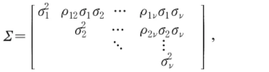
multivariate WSD Method.

Assume that

_ν

-variate random vector

_{X = ( X}

₁

_,…,

X

ν

)

^T is distributed with mean vector

_{μ = (μ}

₁

_,…,μ

_ν

₎

^T and variance-covariance matrix

Σ = ꀎ

ꀚ

︳︳

ꀏ

ꀛ

︳︳

︳︳ σ

²1

ρ

12

σ

1

σ

2

… ρ

1ν

σ

1

σ

ν

σ

²2

… ρ

2ν

σ

2

σ

ν

⋱ ⋯

σ

²ν

, (1)

where ‘

_T

’ denotes the transpose of a vector or matrix,

_σ

_j is the standard deviation of

_X

_j, and

_ρ

_ij is the correlation coefficient of

_X

_i and

_X

_j. For the approximation such as < Figure 1(c)>, the variance- covariance matrix should be adjusted as follows:

_Σ

^W

_{= W Σ W =}

ꀎ

ꀚ

︳︳

ꀏ

ꀛ

︳︳

︳︳ ( σ

^W1

)

²

ρ

12

σ

^W1

σ

^W2

… ρ

1ν

σ

^W1

σ

^Wν

( σ

^W2

)

²

… ρ

2ν

σ

^W2

σ

^Wν

⋱ ⋯ ( σ

^Wν

)

²

, (2)

where

W = diag { W

1

,…,W

ν

}

,

W

j

= { ^2P 2( 1 - P

^j

^,

j

), otherwise , ^{if X}

^j

^{> μ}

^j

^,

(3)

σ

^Wj

= W

j

σ

j, and

_P

_j

_{= Pr { X}

_j

_≤μ

_j

_}

. If

_X

_j is greater than

_μ

_j, the PDF related to

_X

_j is modified by adjusting the

_j

th row and column of the variance- covariance matrix using upper deviation

_2P

_j

_σ

_j in place of

_σ

_j. Otherwise, the

_j

th row and column of the variance-covariance matrix is adjusted using lower deviation

_{2( 1 - P}

_j

_{) σ}

_j. Note that correlation matrix

ρ = { ρ

_ij

}

does not change after the variance-covariance matrix is adjusted. This WSD method approximates the original PDF with segments from

₂

^ν multivariate normal distributions. < Figure 1(c)> is obtained with four bivariate normal distributions with the same mean vector

_{μ = (μ}

_X

_,μ

_Y

₎

^T but different variance-covariance matrices as follows:

Σ

1

= [ ^ρ

^XY

^{⋅2( 1 - P} ^{{ 2( 1 - P}

^X^X

^)σ ^{) σ}

^X^X

^⋅2P ^}

² ^Y

^σ

^Y

^ρ

^XY

^{⋅2( 1 - P} ^{{ 2P}

^Y

^σ

^X

^)σ

^Y

^}

^X²

^⋅2P

^Y

^σ

^Y

]

^,

Σ

₂

= [ ^ρ

^XY

^⋅2P ^{2P

^X^X

^σ ^σ

^X^X

^⋅2P ^}

² ^Y

^σ

^Y

^ρ

^XY

^⋅2P ^{2P

^X^Y

^σ ^σ

^X^Y

^⋅2P ^}

² ^Y

^σ

^Y

]

^,

Σ3=

[

^ρ^XY^{⋅2( 1 - P}^{{ 2( 1 - P}^X^)σ^X^X^{⋅2( 1 - P}^)σ^X^}² ^Y^)σ^Y^ρ^XY^{⋅2( 1 - P}^{{ 2( 1 - P}^X^)σ^X^Y^{⋅2( 1 - P}^)σ^Y^}² ^Y^)σ^Y

]

^,

Σ

4

= [ ^ρ

^XY

^⋅2P ^{2P

^X

^σ

^X

^⋅2(1-P

^X

^σ

^X

^}

² ^Y

^)σ

^Y

^ρ

^XY

^⋅2P ^{2(1-P

^X

^σ

^X

^⋅2(1-P

^Y

^)σ

^Y

^}

² ^Y

^)σ

^Y

]

^.

Since the WSD method approximates the PDF of the original distribution using normal distributions, the standard statistical methods based on the normality

(4)

assumption can be used with the approximated distribution.

3. Multivariate PCIs Based on the WSD Method

3.1 _T

²

Approach

We now propose multivariate

_T

² WSD PCIs. The

T

² statistic is often used in multivariate control charts. The univariate

_C

_pk is defined as the ratio of the distance of the specification limits from the process mean to the actual process spread

_3σ

_X:

_C

_pk

_{= min} { ^{USL -μ} ^3σ

^X ^X

^, ^{LSL -μ} ^3σ

^X ^X

}

_{= min} { ^USL ³

^Z

^, ^LSL ³

^Z

} ^,

⁽⁴⁾

where

_USL

_Z and

_LSL

_Z are the standardized distances from the mean to the upper and lower specification limits, respectively, and the number 3 means the 99.865th percentile of the standard normal distribution which is the same as

_χ

²_0.0027

₍₁₎

. Therefore, formula (4) can be extended to the multivariate case as follows:

C

_pk;T²

= min { ^L ^χ

^T²^0.0027¹

^ρ

^{- 1}

^(ν) ^L

¹

^,…, ^L ^χ

^T²²^0.0027^ν

^ρ

^{- 1}

^(ν) ^L

²^ν

}

= min { ^χ

²^0.0027

^L

^T²

^(ν)

^,1

^,…, ^χ

²

^L

^0.0027^T²^,2

^(ν)

^ν

} ^,

⁽⁵⁾

where

_L

_i is the coordinates of edge

_i

among

₂

^ν edges of the hypercube made by standardized specification limits

_USL

_Z

k

=( USL

_k

- μ

_k

)/σ

_k and

LSL

_Z_k

= ( LSL

k

- μ

k

)/σ

k,

k = 1,2,…,ν

. The order of edges is meaningless, but we assume that

L

1

= (USL

Z1

,…,USL

Zν

)

^T and

_L

₂ν

=(LSL

Z1

,…, LSL

Zν

)

^T. For example, if

_ν=2

,

_L

₁

_{= (USL}

_Z

1

, USL

_Z₂

)

^T and

_L

₄

_{= (LSL}

_Z

1

,LSL

_Z₂

)

^T, and

_L

₂

₌

( USL

_Z₁

,LSL

_Z₂

)

^T and

_L

₃

_{= (LSL}

_Z

1

,USL

_Z₂

)

^T or

L

2

= (LSL

Z1

,USL

Z2

)

^T and

_L

₃

_{= ( USL}

_Z

1

,LSL

Z2

)

^T. If all the correlation coefficients are positive, only

_L

₁ and

_L

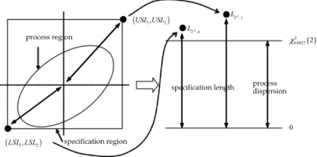
₂ν can be considered since they have the shortest distances from the mean. < Figure 2 >

describes the

_T

² approach for a bivariate distribution with a positive correlation, and shows that

_C

_pk;T2 is the ratio the standardized specification lengths

_L

_T2,1

and

_L

_T2,4 to the process dispersion

_χ

²_0.0027

₍₂₎

.

specification region process region

● (USL USL1, 2)

● (LSL LSL1, 2)

( )

2 0.00272 χ

0

●

specification length process dispersion

2,1

LT 2,4

LT

Figure 2. Concept of _T

² approach.

When the distribution is skewed, the WSD method can be applied, so that formula (5) can be extended to

C

^WSD_pk;T²

= min { ^L ^χ

^W¹²^0.0027^T

^ρ

^{- 1}

^(ν) ^L

^W¹

^,…, ^L ^χ

^W²²^0.0027^T^ν

^ρ

^{- 1}

^(ν) ^L

^W²^ν

}

= min { ^χ

²^0.0027

^L

^W^T²

^(ν)

^,1

^,…, ^χ

²

^L

^0.0027^W^T²^,2

^(ν)

^ν

} ^,

⁽⁶⁾

where the

_k

th component of

_L

^W_i is

_USL

_ZW

k

=(USL

_k

- μ

_k

)/σ

^W_k or

_LSL

_ZW

k

= ( LSL

k

- μ

_k

)/σ

^W_k,

k = 1,2,…,ν

.

3.2 Modified Process Region Approach

Hubele et al. (1991) proposed a 'modified process region approach' which defines a multivariate PCI as the ratio of the volume of engineering tolerance region to the volume of modified process region. < Figure 3 >

illustrates the concept of the method. The modified process region can be obtained by drawing the smallest rectangle around the elliptical probability contour. The edges of the rectangle are defined as the upper and lower process limits,

_UPL

_i and

_LPL

_i,

i = 1,…,ν

, determined by solving the system of equations of first derivatives, with respect to

_X

_i, of the quadratic form

( X - μ )

^T

Σ

^{- 1}

( X - μ ) = χ

²_0.0027

(ν )

.

The solutions to the equation provide the upper and lower limits as follows:

UPL

_i

= μ

_i

+ χ

²_0.0027

( ν )⋅det( Σ

^{- 1}_i

) det( Σ

^{- 1}

) ,

(7)

LPL

i

= μ

i

- χ

²0.0027

( ν )⋅det( Σ

^{- 1}i

) det( Σ

^{- 1}

) ,

where

_det(⋅)

is the determinant of a matrix and

_Σ

_i is the matrix obtained from

_Σ

by deleting row

_i

and column

_i

. The approach defines the multivariate PCI

C

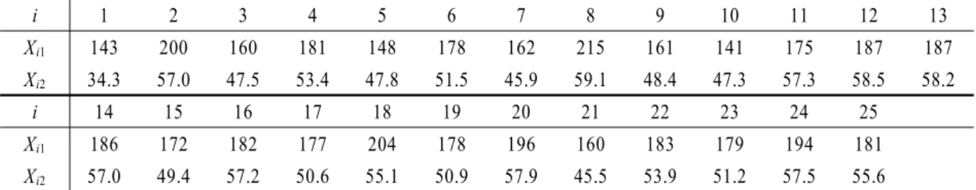
p;M as

(5)

Table 1. Data for the example

i 1 2 3 4 5 6 7 8 9 10 11 12 13

X

i1

143 200 160 181 148 178 162 215 161 141 175 187 187 X

i2

34.3 57.0 47.5 53.4 47.8 51.5 45.9 59.1 48.4 47.3 57.3 58.5 58.2

i 14 15 16 17 18 19 20 21 22 23 24 25

X

i1

186 172 182 177 204 178 196 160 183 179 194 181 X

i2

57.0 49.4 57.2 50.6 55.1 50.9 57.9 45.5 53.9 51.2 57.5 55.6

C

p;M

= [

^{i = 1}

^∏

^ν

( ^UPL ^USL

ⁱⁱ

^{- LSL} ^-LPL

ⁱⁱ

)]

^1/ν^. ⁽⁸⁾

If the process mean and specification midpoint are incorporated in the PCI and the specification limits are standardized,

_C

_pk;M can be defined as

C

_pk;M

= [

^{i = 1}

^∏

^ν

^min { ^UPL ^USL

^Z^Zⁱⁱ

^, ^LPL ^LSL

^Z^Zⁱⁱ

}]

^1/ν^, ⁽⁹⁾

where

UPL

Zi

= χ

²0.0027

(ν) ⋅det( ρ

^{- 1}i

) det( ρ

^{- 1}

) ,

LPL

Zi

= - χ

²0.0027

(ν) ⋅det( ρ

^{- 1}i

)

det( ρ

^{- 1}

) =- UPL

Zi

.

(10)

process region

specification region modified process region

Figure 3. concept of modified process region

approach.

When the distribution is skewed, the WSD method can be applied.

_USL

^W_Z

i and

_LSL

^W_Z

i replace

_USL

_Z

i

and

_LSL

_Z

i in formula (10), respectively, and hence

C

^WSD_pk;M is defined as

C

^WSDpk;M

= [

^{i = 1}

^∏

^ν

^min { ^USL ^UPL

^W^Z^Zⁱⁱ

^, ^LSL ^LPL

^W^Z^Zⁱⁱ

}]

^1/ν^{. (11)}

3.3 Estimation of Parameters

To use PCIs in practice, the parameters must be estimated. If a random sample of size

_n

is obtained,

μ

and

_Σ

can be estimated by the sample mean

X = 1 n ∑

n i = 1

X

i

and the sample variance-covariance matrix

S = 1 n - 1 ∑

n

i = 1

( X

_i

- X )( X

_i

- X )

^T,

respectively. The correlation coefficient of

_j

th and

k

th random variables

_ρ

_jk can be estimated by

ˆ ρ

jk

= S

ij

S

jj

S

kk

,

where

_S

_jkis the (

_j,k

)th element of

_S

.

_P

_j can be estimated by the number of observations less than or equal to the sample mean of

_j

th quality characteristic

X

j as

ˆ P

j

= 1 n ∑

n

i = 1

I( X

j

- X

ij

)

,

where

_I(x)=1

if

_x≥0

or

_I(x)=0

otherwise.

3.4 An Illustrative Example

We illustrate the use of the proposed WSD PCIs with the bivariate process data in Sultan (1986) dealing with 25 observations of the Brinell hardness (

_X

₁) and the tensile strength (

_X

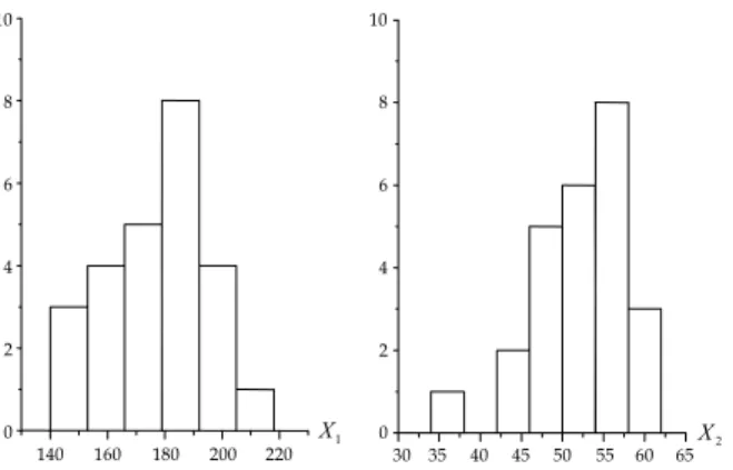
₂) of a process.

These data were also used by Chan et al. (1988), Chen (1994), and Wang and Chen (1998-99). < Table 1 >

presents the data, and < Figure 4 > depicts the histograms of

_X

₁ and

_X

₂ and shows that the marginal distributions of

_X

₁ and

_X

₂ are slightly skewed to the left. The specification limits for

_X

₁ and

X

₂ were set at (112.7, 2451.3) and (32.7, 73.3), respectively.

(6)

140 160 180 200 220 0

2 4 6 8 10

X

1

30 35 40 45 50 55 60 65

0 2 4 6 8 10

X

2

Figure 4. Histograms of data in <table 1>.

From the data,

_X

₁

_{= 177.2}

,

_X

₂

_{= 52.32}

,

^ˆ _σ

₁

₌

18.38

,

^ˆ _σ

₂

_{= 5.80}

,

^ˆ _ρ

₁₂

_{= 0.80}

,

^ˆ _P

₁

_{= 0.40}

, and

ˆ P

2

=0.48

. We can obtain

_LSL

_Z

1

= ( LSL

₁

- X

₁

)/ σ ˆ

₁

₌ ( 112.7 - 17 7.2)/18.38 =- 3.51

,

_USL

_Z

1

= 3.49

,

_LSL

_Z

2

=- 3.38

,

_USL

_Z

2

= 3.62

,

_LSL

^W_Z

1

= LSL

Z₁

/2( 1 - P ˆ

1

)

=- 2.93

,

_USL

^W_Z

1

= 4.36

,

_LSL

^W_Z

2

=- 3.25

,

_USL

^W_Z

2

= 3.77

. Also,

L

_T²_{, 1}

= L

^T1

ρ

^{- 1}

L

1

= [ -3.51 - 3.38 ]

[

0.8 ¹ ^0.8 1

][

^{- 3.51} - 3.38

]

= 13.57

,

L

_T²_{, 4}

= L

^T4

ρ

^{- 1}

L

4

= [ 3.49 3.62 ]

[

0.8 ¹ ^0.8 1

][

^3.49 3.62

]

= 14.08

,

L

^W_T²_{, 1}

= L

^W1^T

ρ

^{- 1}

L

1

= [ - 2.93 - 3.25 ]

[

0.8 ¹ ^0.8 1

][

^{- 2.93} - 3.25

]

= 10.87

,

L

^W_T²_{, 4}

= L

^W4^T

ρ

^{- 1}

L

4

= [ 4.36 3.77 ]

[

0.8 ¹ ^0.8 1

][

^4.36 3.77

]

= 19.23

,

UPL

Zi

= χ

²0.0027

(2) ⋅det( ρ

^{- 1}i

) det( ρ

^{- 1}

)

₌ ^11.83⋅2.78

2.78 = 3.44

and

_LPL

_Z

i

=- UPL

Zi

=- 3.44

for

_{i = 1,2}

. Then the estimated PCIs are:

The

_T

² approach ―

ˆ C

pk;T²

= min { ^χ

²^0.0027

^L

^T²^{, 1}

⁽²⁾ ^, ^χ

²^0.0027

^L

^T²^{, 4}

⁽²⁾ }

_{= min}

{

^13.57 11.83 , 14.08 11.83

}

= min { 1.07 , 1.09 } = 1.07

ˆ C

^WSD

pk;T²

= min { ^χ

²^0.0027

^L

^W^T²^{, 1}

⁽²⁾ ^, ^χ

²^0.0027

^L

^W^T²

⁽²⁾

^{, 4}

}

_{= min}

{

^10.87 11.83 , 19.23 11.83

}

= min { 0.96 , 1.27 } = 0.96

The modified process region approach ―

ˆ C

pk;M

= [

^{i = 1}

^∏

²

^min { ^UPL ^USL

^Z^Zⁱⁱ

^, ^LPL ^LSL

^Z^Zⁱⁱ

}]

^1/2

₌ [ ^min { ^3.49 3.44 , - 3.51 - 3.44 } ^⋅

_min { ^3.62 3.44 , - 3.38 - 3.44 }]

^1/2

= [ 1.01⋅0.98]

^1/2

= 0.99

ˆ C

WSD

pk;M

= [

^{i = 1}

^∏

²

^min { ^USL ^UPL

^W^Z^Zⁱⁱ

^, ^LSL ^LPL

^W^Z^Zⁱⁱ

}]

^1/2

₌ [ ^min { ^4.36 3.44 , - 2.93 - 3.44 } ^⋅

_min { ^3.77 3.44 , - 3.25 - 3.44 }]

^1/2

= [ 0.85⋅0.94]

^1/2

= 0.89 ˆ C

^WSD

pk;T² and

^ˆ _C

^WSD_pk;M are smaller than

^ˆ _C

_pk;T2 and

ˆ C

pk;M, respectively, and this shows that the process is less satisfactory than

^ˆ _C

_pk;T2 and

^ˆ _C

_pk;M indicate.

4. Performance of the W SD PCIs

The performances of the proposed PCIs are studied when the distribution is multivariate normal, multivariate lognormal, Hougaard's bivariate Weibull, or Cheriyan and Ramabhadran's bivariate gamma. See Kotz et al. (2000) for detailed discussions on theses distributions. For all cases, it is assumed that

USL

i

= 3

and

_LSL

_i

_{=- 3}

, and the distribution is shifted and scaled to produce the same value of

_μ

_i

_{= 0}

and

_σ

_i

_{= 1}

,

_{i = 1,…,ν}

.

< Tables 2 > gives

_C

_pk;T2, and

_C

_pk;M as the sample size

_n

increases when the distribution is bivariate normal and the correlation coefficient

_ρ

is nonnegative.

It also gives nonconforming proportion per million (

_NPM

) and

_MC

_p.

_MC

_p is calculated by

_-(1/3)Φ

^{- 1}

( ( NPM/2) ×10

^{- 6}

)

since

_NPM×10

^{- 6}

= 2Φ( - 3 C

p

)

(7)

Table 2. _NPM

,

_MC

_p,

_C

_pk;T2 and

_C

_pk;M for bivariate normal distributions

ρ NPM MC

p

n = 50 n = 100 n = 200 n = ∞

C

_pk;T²

C

pk;M

C

_pk;T²

C

pk;M

C

_pk;T²

C

pk;M

C

_pk;T²

C

pk;M

0.0 0.1 0.2 0.3 0.4 0.5 0.6 0.7 0.8 0.9

5,392 5,389 5,377 5,352 5,308 5,236 5,120 4,940 4,655 4,179

0.928 0.928 0.928 0.928 0.929 0.931 0.933 0.937 0.943 0.955

1.233 1.174 1.123 1.077 1.036 1.000 0.969 0.938 0.911 0.885

0.850 0.850 0.850 0.851 0.850 0.851 0.852 0.851 0.852 0.851

1.227 1.168 1.118 1.073 1.032 0.998 0.964 0.935 0.909 0.882

0.855 0.854 0.855 0.854 0.854 0.855 0.854 0.855 0.856 0.854

1.226 1.168 1.118 1.073 1.033 0.997 0.965 0.936 0.909 0.885

0.859 0.859 0.859 0.859 0.859 0.859 0.859 0.859 0.859 0.859

1.234 1.176 1.126 1.082 1.043 1.007 0.975 0.946 0.919 0.895

0.872 0.872 0.872 0.872 0.872 0.872 0.872 0.872 0.872 0.872 n = ∞ : parameters-known case

Table 3. _NPM

,

_MC

_p,

_C

_pk;T2,

_C

^WSD_pk;T2,

_C

_pk;M and

_C

^WSD_pk;M for bivariate distributions (parameters known)

(a) _{ρ = 0.3}

dist. (γ

₁

,γ

₂

) NPM MC

p

C

_pk;T²

C

^WSD_pk;T²

C

pk;M

C

^WSDpk;M

lognormal

(1,1) (1,2) (1,3) (2,2) (2,3) (3,3)

20,295 25,883 27,700 31,332 33,095 34,841

0.774 0.743 0.734 0.718 0.710 0.703

1.082 1.082 1.082 1.082 1.082 1.082

0.962 0.927 0.907 0.889 0.868 0.845

0.872 0.872 0.872 0.872 0.872 0.872

0.776 0.746 0.727 0.717 0.699 0.682

Weibull

(1,1) (1,2) (1,3) (2,2) (2,3) (3,3)

19,344 27,495 30,221 35,243 37,948 40,513

0.780 0.735 0.722 0.702 0.692 0.683

1.082 1.082 1.082 1.082 1.082 1.082

0.948 0.904 0.880 0.856 0.829 0.801

0.872 0.872 0.872 0.872 0.872 0.872

0.764 0.726 0.702 0.690 0.667 0.645

gamma

(1,1) (1,2) (1,3) (2,2) (2,3) (3,3)

19,602 27,168 31,228 33,245 37,270 39,731

0.778 0.736 0.718 0.710 0.694 0.686

1.082 1.082 1.082 1.082 1.082 1.082

0.955 0.908 0.876 0.856 0.820 0.781

0.872 0.872 0.872 0.872 0.872 0.872

0.770 0.729 0.696 0.690 0.659 0.630

under the normality assumption, where

_Φ(⋅)

is the

cumulative standard normal distribution function. If the value of PCI is close to that of

_MC

_p or

_MC

_pk, the PCI can be considered to describe the process capability very well in terms of nonconforming proportion.

The Table shows that:

i) If the parameters are known (

_{n = ∞}

),

_MC

_p slightly increases as the correlation coefficient

_ρ

increases but

_C

_pk;T2 decreases and

_C

_pk;M does not change. Also,

_C

_pk;T2 overestimates the process capability when the correlation is low and

underestimates it when the correlation is high, and

_C

_pk;M underestimates it for all ranges of correlation. For highly correlated normal populations,

_C

_pk;T2 performs better than

_C

_pk;M, and vise versa.

ii) If the parameters are unknown (

n = 50,100,200

), the biases of

^ˆ _C

_pk;T2 and

^ˆ _C

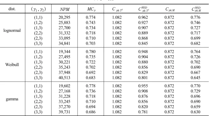
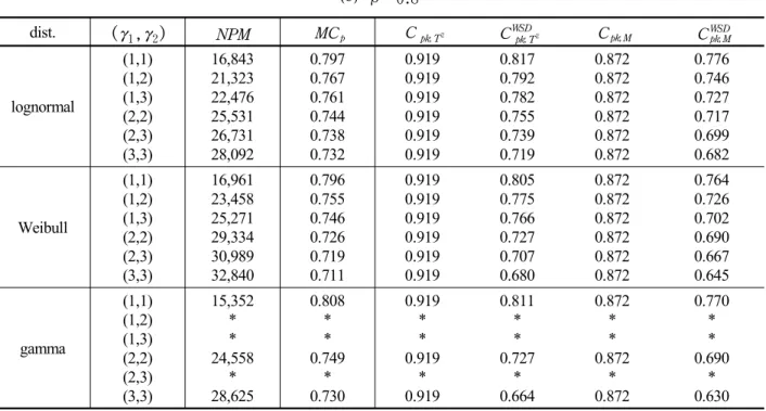
_pk;M are negative.

< Table 3 > and < Table 4 > give

_C

_pk;T2,

_C

^WSD_pk;T2,

C

_pk;M, and

_C

^WSD_pk;M for bivariate lognormal, Weibull, and gamma distributions with correlation

_{ρ = 0.3}

or

(8)

(b) _{ρ = 0.8}

dist. (γ

₁

,γ

₂

) NPM MC

p

C

_pk;T²

C

^WSD_pk;T²

C

pk;M

C

^WSD_pk;M

lognormal

(1,1) (1,2) (1,3) (2,2) (2,3) (3,3)

16,843 21,323 22,476 25,531 26,731 28,092

0.797 0.767 0.761 0.744 0.738 0.732

0.919 0.919 0.919 0.919 0.919 0.919

0.817 0.792 0.782 0.755 0.739 0.719

0.872 0.872 0.872 0.872 0.872 0.872

0.776 0.746 0.727 0.717 0.699 0.682

Weibull

(1,1) (1,2) (1,3) (2,2) (2,3) (3,3)

16,961 23,458 25,271 29,334 30,989 32,840

0.796 0.755 0.746 0.726 0.719 0.711

0.919 0.919 0.919 0.919 0.919 0.919

0.805 0.775 0.766 0.727 0.707 0.680

0.872 0.872 0.872 0.872 0.872 0.872

0.764 0.726 0.702 0.690 0.667 0.645

gamma

(1,1) (1,2) (1,3) (2,2) (2,3) (3,3)

15,352

*

* 24,558

* 28,625

0.808 *

* 0.749

* 0.730

0.919 *

* 0.919

0.811 *

* 0.727

* 0.664

0.872 *

* 0.872

0.770 *

* 0.690

* 0.630

*: not applicable

Table 4. _C

_pk;T2,

_C

^WSD_pk;T2,

_C

_pk;M and

_C

^WSD_pk;M for bivariate distributions(parameters unknown)

(a) _{ρ = 0.3}

dist. (γ

₁

,γ

₂

) ^{n = 50} ^{n = 100} ^{n = 200}

C

_pk;T²

C

^WSD_pk;T²

C

pk;M

C

^WSDpk;M

C

_pk;T²

C

^WSD_pk;T²

C

pk;M

C

^WSDpk;M

C

_pk;T²

C

^WSD_pk;T²

C

pk;M

C

^WSDpk;M

lognormal (1,1) (1,2) (1,3) (2,2) (2,3) (3,3)

1.095 1.111 1.143 1.313 1.160 1.187

1.026 1.011 1.019 0.998 1.001 1.007

0.860 0.869 0.888 0.882 0.898 0.914

0.794 0.778 0.777 0.765 0.762 0.758

1.082 1.093 1.111 1.106 1.119 1.138

0.995 0.973 0.968 0.948 0.939 0.935

0.860 0.867 0.876 0.874 0.881 0.892

0.788 0.766 0.756 0.744 0.733 0.725

1.077 1.083 1.091 1.090 1.097 1.108

0.980 0.950 0.936 0.920 0.904 0.892

0.861 0.865 0.868 0.868 0.873 0.878

0.783 0.756 0.741 0.731 0.716 0.704

Weibull

(1,1) (1,2) (1,3) (2,2) (2,3) (3,3)

1.085 1.108 1.141 1.127 1.158 1.193

1.002 0.982 0.984 0.953 0.953 0.958

0.856 0.870 0.886 0.880 0.897 0.918

0.782 0.760 0.751 0.735 0.726 0.722

1.076 1.089 1.102 1.101 1.118 1.135

0.975 0.942 0.927 0.906 0.893 0.881

0.857 0.863 0.871 0.871 0.880 0.891

0.775 0.743 0.725 0.713 0.698 0.685

1.074 1.080 1.090 1.086 1.096 1.105

0.960 0.922 0.905 0.880 0.862 0.841

0.859 0.863 0.869 0.866 0.872 0.877

0.769 0.735 0.716 0.701 0.683 0.665

gamma

(1,1) (1,2) (1,3) (2,2) (2,3) (3,3)

1.091 1.115 1.152 1.135 1.174 1.211

1.103 0.992 0.987 0.960 0.954 0.943

0.858 0.869 0.887 0.881 0.901 0.920

0.788 0.762 0.744 0.737 0.722 0.705

1.079 1.092 1.111 1.106 1.119 1.141

0.984 0.950 0.930 0.909 0.882 0.861

0.858 0.864 0.874 0.872 0.877 0.890

0.780 0.747 0.722 0.714 0.687 0.667

1.076 1.082 1.094 1.089 1.098 1.109

0.970 0.928 0.905 0.883 0.854 0.822

0.860 0.863 0.869 0.867 0.872 0.877

0.776 0.737 0.710 0.702 0.675 0.649 ρ = 0.8

and various skewnesses (

_γ

₁

_{, γ}

₂).

_NPM

and

MC

_p are also given in < Table 3 >. The tables show that:

i) When the parameters are known,

_MC

_p decreases

as skewness increases and

_C

^WSD_pk;T2 and

_C

^WSD_pk;M reflect such a phenomenon, i.e., they decrease as skewness becomes large whereas

_C

_pk;T2 and

C

_pk;M remain constant; <Table 3>

(9)

(b) _{ρ = 0.8}

dist. (γ

₁

,γ

₂

) ^{n = 50} ^{n = 100} ^{n = 200}

C

_pk;T²

C

^WSD_pk;T²

C

_pk;M

C

^WSD_pk;M

C

_pk;T²

C

^WSD_pk;T²

C

_pk;M

C

^WSD_pk;M

C

_pk;T²

C

^WSD_pk;T²

C

_pk;M

C

^WSD_pk;M

lognormal (1,1) (1,2) (1,3) (2,2) (2,3) (3,3)

0.928 0.950 0.983 0.968 0.997 1.026

0.879 0.878 0.888 0.870 0.877 0.888

0.862 0.874 0.889 0.887 0.902 0.923

0.797 0.784 0.780 0.772 0.769 0.771

0.916 0.932 0.948 0.941 0.959 0.973

0.850 0.840 0.836 0.816 0.814 0.809

0.860 0.869 0.875 0.875 0.886 0.896

0.788 0.769 0.756 0.746 0.738 0.731

0.913 0.921 0.932 0.928 0.938 0.948

0.834 0.815 0.811 0.788 0.780 0.769

0.861 0.865 0.871 0.870 0.877 0.883

0.783 0.757 0.744 0.733 0.721 0.709

Weibull

(1,1) (1,2) (1,3) (2,2) (2,3) (3,3)

0.923 0.947 0.995 0.968 1.007 1.032

0.866 0.857 0.870 0.839 0.848 0.847

0.858 0.870 0.891 0.883 0.903 0.922

0.785 0.761 0.757 0.740 0.736 0.728

0.914 0.928 0.951 0.939 0.956 0.975

0.836 0.817 0.815 0.783 0.774 0.766

0.858 0.865 0.876 0.872 0.881 0.894

0.776 0.746 0.732 0.716 0.700 0.688

0.912 0.918 0.931 0.925 0.937 0.944

0.821 0.794 0.791 0.755 0.744 0.724

0.861 0.863 0.870 0.867 0.875 0.879

0.770 0.735 0.717 0.702 0.686 0.667

gamma

(1,1) (1,2) (1,3) (2,2) (2,3) (3,3)

0.924 *

* 0.960

* 1.009

0.868 *

* 0.820

* 0.791

0.861 *

* 0.886

* 0.922

0.793 *

* 0.742

* 0.709

0.915 *

* 0.931

* 0.959

0.841 *

* 0.771

* 0.727

0.859 *

* 0.871

* 0.891

0.783 *

* 0.715

* 0.669

0.913 *

* 0.921

* 0.938

0.827 *

* 0.750

* 0.698

0.861 *

* 0.867

* 0.879

0.778 *

* 0.702

* 0.651

Table 5. _NPM

,

_MC

_p,

_C

pk;T²,

_C

^WSD

pk;T²,

_C

_pk;M and

_C

^WSD_pk;M for 4-variate lognormal distributions (parameters known)

case ( γ

₁

,γ

₂

,γ

_3,

γ

₄

) NPM MC

_p

C

_pk;T²

C

^WSD_pk;T²

C

_pk;M

C

^WSDpk;M

1 (1.0,0.5,1.0,0.5) (1.5,1.0,1.0,1.5) (1.5,1.5,2.5,2.5) (0.5,2.5,2.0,1.5)

15,916 24,016 27,417 22,865

0.804 0.752 0.735 0.759

1.128 1.128 1.128 1.128

1.030 0.980 0.933 0.973

0.744 0.744 0.744 0.744

0.680 0.647 0.614 0.633

2 (1.0,0.5,1.0,0.5) (1.5,1.0,1.0,1.5) (1.5,1.5,2.5,2.5) (0.5,2.5,2.0,1.5)

13,352 19,631 22,308 19,230

0.825 0.778 0.762 0.780

0.865 0.865 0.865 0.865

0.810 0.754 0.712 0.755

0.744 0.744 0.744 0.744

0.680 0.647 0.614 0.633

ii) When the parameters are unknown,

_C

_pk;T2 and

C

_pk;M increase as skewness becomes large, whereas

_C

^WSD_pk;T2 and

_C

^WSD_pk;M decrease in most cases. All PCIs are overestimated especially when the sample size is small; < Table 4 >

iii)

_C

^WSD_pk;M is closer to

_MC

_p in < Table 3(a)>, and

C

^WSD_pk;T² is closer to

_MC

_p in < Table 3(b)> except for

_{( γ}

₁

_,γ

₂

_{) = ( 1,2)}

. Also, < Table 4 > and addi- tional extensive study we have conducted indicate that

_C

^WSD_pk;T2 is closer to

_MC

_p for highly correlated populations as sample size becomes large, and vise versa. This shows that the

_T

² approach is superior to the modified process region approach for highly correlated populations

in most cases, and vise versa.

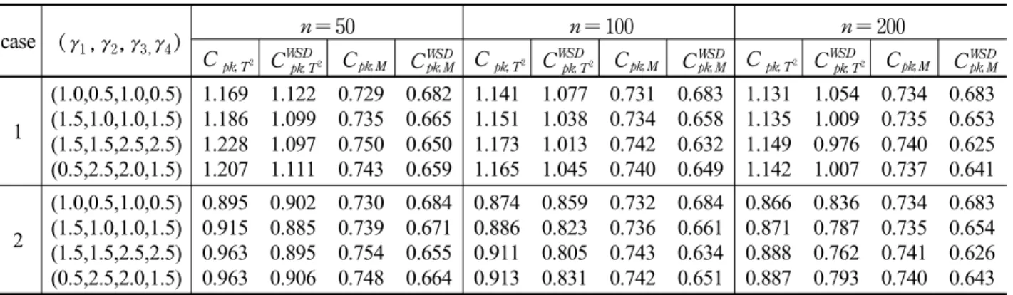
< Table 5 > and < Table 6 > present PCIs for two 4-variate lognormal distributions, where case 1 uses

ρ

1 describing low positive correlations (

_ρ

_ij

_{< 0.5}

) and case 2 uses

_ρ

₂ containing high correlations (

_ρ

_ij

_≥0.5

) as follows:

ρ

1

= ꀎ

ꀚ

︳︳

ꀏ

ꀛ

︳︳

︳︳ 1 0.2 0.3 0.1

1 0.2 0.4 1 0.3 1

,

ρ

₂

= ꀎ

ꀚ

︳︳

ꀏ

ꀛ

︳︳

︳︳ 1 0.8 0.6 0.7

1 0.8 0.5 1 0.6 1

.

Multivariate Process Capability Indices for Skewed Populations with Weighted Standard Deviations

1

2†

1

2

1

2

1

2

T

Keywords: process capability index, skewed population, weighted standard deviation, T

†Corresponding author : Professor Do Sun Bai, Department of Industrial Engineering, Korea Advanced Institute of Science and Technology, Daejon, Korea, 305-701, Fax : 82-42-869-3110, e-mail : [email protected]

Received November 2002; revision received February 2003; accepted February 2003.

1. Introduction

C

C

USL

LSL

MC

al. (1994) considered geometric dimensioning and

T

T

T

2. W eighted Standard Deviation(W SD) M ethod

σ

σ

σ

μ

σ

σ

σ

= P

σ

σ

= ( 1 - P

) σ

P

= Pr { X≤μ

}

μ

2σ

2σ

T

X

Y

X

Y

( X,Y )

X

Y

(a) iso-PDF contours of skewed distribution

(b) iso-PDF contour of normal distribution

(c) iso-PDF contour approximated with WSD method MVN(μ, Σ): multivariate normal distribution with

mean vector μ and variance-covariance matrix Σ

Figure 1. Iso-PDF contours and concept of

ν

X = ( X

,…,

X

)

μ = (μ

,…,μ

)

Σ = ꀎ

ꀚ

︳ ︳

︳ ︳

︳ ︳

︳ ︳

︳ ︳

ꀏ

ꀛ

︳ ︳

︳ ︳

︳ ︳

︳ ︳

︳ ︳ σ

ρ

σ

σ

¹

^2†

²

¹

²

_T

Keywords: process capability index, skewed population, weighted standard deviation, _T

_C

_C

_USL

_LSL

_MC

_T

_T

_T

_σ

_σ

_σ

_μ

_σ

_σ

_σ

_{= P}

_σ

_σ

_{= ( 1 - P}

_{) σ}

_μ

_2σ

_T

_X

_Y

_X

_Y

_{( X,Y )}

_X

_Y

_ν

_{X = ( X}

_,…,

_{μ = (μ}

_,…,μ

₎

︳︳

︳︳

︳︳

︳︳

︳︳

︳︳

︳︳

︳︳

︳︳

︳︳ σ

_T

_σ

_X

_ρ

_X

_X

_Σ

_{= W Σ W =}

︳︳

︳︳

︳︳

︳︳

︳︳

︳︳

︳︳

︳︳

︳︳

︳︳ ( σ

= { ^2P 2( 1 - P

^,

), otherwise , ^{if X}

^{> μ}

^,

_P

_{= Pr { X}

_≤μ

_}