수직다관절형 아암의 운동학적 모델링 및 관절공간 모션제어에 관한 연구
A Study on Kinematics Modeling and Motion Control Algorithm Development in Joint for Vertical Type
Articulated Robot Arma
조상영1*, 김민성1, 양준석1, 원종범2, 한성현3
Sang-Young Jo1*, Min-Seong Kim1, Jun-Seok Yang1, Jong-Bum Won2, Sung-Hyun Han3
<Abstract>
In this paper, we propose a new technique to the design and real-time control of an adaptive controller for robotic manipulator based on digital signal processors. The Texas Instruments DSPs(TMS320C80) chips are used in implementing real-time adaptive control algorithms to provide enhanced motion control performance for dual-arm robotic manipulators. In the proposed scheme, adaptation laws are derived from model reference adaptive control principle based on the improved Lyapunov second method.
The proposed adaptive controller consists of an adaptive feed-forward and feedback controller and time-varying auxiliary controller elements. The proposed control scheme is simple in structure, fast in computation, and suitable for real-time control.
Moreover, this scheme does not require any accurate dynamic modeling, nor values of manipulator parameters and payload. Performance of the proposed adaptive controller is illustrated by simulation and experimental results for a dual arm robot manipulator with eight joints. joint space and cartesian space.
Keywords : Adaptive Control, Seven Joints Robot, Real Time Control, Implementation, Lyapunov
1*정회원, 교신저자, 경남대학교 첨단공학과 (E-mail: [email protected]) 2 정회원, (주)SMEC, 대표
3 정회원, 경남대학교 기계공학부 교수 工博
1*Dept. of Advanced Engineering, Kyungnam University.
2 SMEC Co., Ltd., CEO
3 Prof., School of Mechanical Engineering, Kyungnam University, Ph. D.
1. INTRODUCTION
Currently there are much advanced techniques that are suitable for servo control of a large class of nonlinear systems including robotic manipulators (P.C.V. Parks, 1966; Y.K.Choi et al., 1986; Y.M.Yoshhiko, 1995). Since the pioneering work of Dubowsky and DesForges (1979), the interest in adaptive control of robot manipulators has been growing steadily (T. C. Hasi, 1986; D.
Koditschck, 1983; A. Koivo et al., 1983; S.
Nicosia et al., 1984). This growth is largely due to the fact that adaptive control theory is particularly well-suited to robotic manipulators whose dynamic model is highly complex and may contain unknown parameters. However, implementation of these algorithms generally involves intensive numerical computations (J. J. Craig, 1988; H.
Berghuis et al., 1993).
Current industrial approaches to the design of robot arm control systems treat each joint of the robot arm as a simple servomechanism. This approach models the time varying dynamics of a manipulator inadequately because it neglects the motion and configuration of the whole arm mechanism. The changes in the parameters of the controlled system are significant enough to render conventional feedback control strategies ineffective. This basic control system enables a manipulator to perform simple positioning tasks such as in the
pick-and-place operation. However, joint controllers are severely limited in precise tracking of fast trajectories and sustaining desirable dynamic performance for variations of payload and parameter uncertainties (R.
Ortega et al., 1989; P. Tomei, 1991). In many servo control applications the linear control scheme proves unsatisfactory, therefore, a need for nonlinear techniques is increasing.
Adaptive and optimal multi variable control methods can track system parameter variations. Dual control, learning, neural networks, genetic algorithms and Fuzzy Logic control methodologies are all among the digital controllers implementable by a DSP (N. Sadegh et al., 1990; Z. Ma et al., 1995).
In addition, DSP's are as fast in computation as most 32-bit microprocessors and yet at a fraction of their prices. These features make them a viable computational tool for digital implementation of advanced controllers. High performance DSPs with increased levels of integration for functional modules have become the dominant solution for digital control systems. Digital signal processors (DSP's) are special purpose microprocessors that are particularly suitable for intensive numerical computations involving sums and products of variables. Digital versions of most advanced control algorithms can be defined as sums and products of measured variables, thus can naturally be implemented by DSP's.
DSPs allow straightforward implementation of advanced control algorithms that result in improved system control.
This paper describes a new approach to the design of adaptive control system and real-time implementation of dual arm robot using digital signal processors for robotic manipulators to achieve the improvement of speed ness, repeating precision, and tracking performance at the joint and cartesian space.
This paper is organized as follows : In Section Ⅱ, the dynamic model of the robotic manipulator is derived. Section Ⅲ derives adaptive control laws based on the model reference adaptive control theory using the improved Lyapunov second method. Section
Ⅳ presents simulation and experimental results obtained for a eight joints robot.
2. System Modeling
The dynamic model of a manipulator-plus- payload is derived and the tracking control p roblem is stated in this section.
Let us consider a non redundant joint robotic manipulator in which the n×1 generalized joint torque vector is related to the n×1 generalized joint coordinate vector by the following nonlinear dynamic equation of motion
(1)
where is the n×n symmetric positive-definite inertia matrix, is the n×1 coriolis and centrifugal torque vector,
and is the n×1 gravitational loading vector. discusses the findings and draws some conclusions.
Equation (1) describes the manipulator dynamics without any payload. Now, let the n×1 vector X represent the end-effector position and orientation coordinates in a fixed task-related cartesian frame of reference. The cartesian position, velocity, and acceleration vectors of the end-effector are related to the joint variables by
(2)
where is the n×1 vector representing the forward kinematics and
is the n×n Jacobian matrix of the manipulator.
Let us now consider payload in the manipulator dynamics. Suppose that the manipulator end-effector is firmly grasping a payload represented by the point mass ∆.
For the payload to move with acceleration
in the gravity field, the end-effector must apply the n×1 force vector given by
∆ (3)
그림1. 6관절 로봇 매니퓰레이터의 적응 제어구조 Fig. 1. Adaptive control scheme of Robotic
Manipulator with eight joint
where g is the n×1 gravitational acceleration vector. The end-effector requires the additional joint torque
) ( ) ( )
(t J q TT t
f =
t (4)
where superscript T denotes transposition.
Hence, the total joint torque vector can be obtained by combining equations (1) and (4) as
(5)
Substituting equations (2) and (3) into equation (5) yields
∆ (6)
Equation (6) shows explicity the effect of payload mass ∆ on the manipulator dynamics. This equation can be written as
∆
∆ ∆
(7)
where the modified inertia matrix
∆ is symmetric and positive-definite. Equation (7) constitutes a nonlinear mathematical model of the manipulator-plus-payload dynamics.
3. Controller Design
The manipulator control problem is to develop a control scheme which ensures that the joint angle vector q(t) tracks any desired reference trajectory qr(t) ,where qr(t) is an n×1 vector of arbitrary time functions. It is reasonable to assume that these functions are twice differentiable, that is, desired angular velocity and angular acceleration
exist and are directly available without requiring further differentiation of . It is desirable for the manipulator control system to achieve trajectory tracking irrespective of payload mass∆.
The controllers designed by the classical linear control scheme are effective in fine motion control of the manipulator in the neighborhood of a nominal operating point
. During the gross motion of the manipulator, operating point and consequently the linearized model parameters vary substantially with time. Thus it is essential to adapt the gains of the feedforward, feedback, and PI controllers to varying operating points and payloads so as to ensure stability and trajectory tracking by the total control laws. The required adaptation laws are developed in this section.
Fig. 1 represents the block diagram of adaptive control scheme for robotic manipulator.
Nonlinear dynamic equation (7) can be written as
∆ ∆
∆ (8)
where , , and are n×n matrices whose elements are highly nonlinear functions of ∆, , and .
In order to cope with changes in operating point, the controller gains are varied with the change of external working condition.
This yields the adaptive control law
(9)
where are feedfor ward time-varying adaptive gains, and
and are the feedback adapti ve gains, and is a time-varying con trol signal corresponding to the nominal operating point term, generated by a feedba ck controller driven by position tracking error E(t) defined as .
On applying adaptive control law (9) to nonlinear model (8) as shown in Fig. 1, the error differential equation can be obtained as
(10)
Defining the 2n×1 position-velocity error vector d(t)=[E(t),E&(t)]T, equation(10) can be written in the state-space form
÷÷ ø ö çç è +æ
÷÷ ø ö çç è + æ
÷÷ ø ö çç è +æ
÷÷ ø ö çç è +æ
÷÷ ø ö çç
è
= æ
6 5
4 2 3
1
) 0 0 (
) 0 ( ) 0 ( ) 0 (
) (
t Z Z q
t Z q t Z q Z t
Z t I
r
r r
n
&
&
&
& d
d
(11)
where,
and
Equation (11) constitutes an adjustable system in the model reference adaptive control frame-work. We shall now define the reference model which embodies the desired performance of the manipulator in terms of the tracking error E(t). The desired performance is that each joint tracking error
be decoupled from the others and satisfy a second-order homogeneous differential equation of the form
(i=1, … , n) (12)
where and are the damping ratio and the undamped natural frequency.
The desired performance of the control system is embodied in the definition of the stable reference model equation (12) as following vector equation (13).
()
) 0 (
2 1
S t S
t In g
g d
d ÷÷
ø ö çç
è æ
-
= -
&
(13)
where S1=diag(vi2) and S2 =diag(2xivi) are constant n×n diagonal matrices,
is the 2n×1 vector of desired position and velocity errors, and the subscript ' g ' denotes the reference model.
Because reference model is stable, equation (13) has Lyapunov function's solution R defined as following equation
(14)
where is symmetric positive definite matrix.
R is symmetric positive definite matrix
defined as ú ú û ù ê ê ë é
3 2
2 1
R R
R R
.
We shall now state the adaptation laws which ensure that, for any reference trajectory , the state of the adjust able system, approaches asymptotically. The controller adaptation laws will be derived using the direct Lyapunov method-based model reference adaptive control technique. The adaptive control problem is to adjust the controller continuously so that, for any , the system state error
approaches asymptotically, i.e. → as
→ ∞.
Let the adaptation error be defined as
, and then from equation(13), the error differential equation(11) can be defined as
÷÷ ø ö çç è æ + -
÷÷ ø ö çç è æ + -
÷÷ ø ö çç è æ + -
÷÷ ø ö çç è æ + -
÷÷ ø ö çç
è æ
- + -
÷÷ ø ö çç
è æ
-
= -
6 5
4 3
2 2 1 1 2
1
0 0
0 0
0 0
q Z q Z
q Z Z
S Z S Z
I S
S I
r r
r
n n
&
&
&
& e
e
(15)
The controller adaptation laws shall be derived by ensuring the stability of error dynamics equation (15). To this end, let us define a scalar positive-definite Lyapunov function as
∆∆
∆∆
∆∆
∆∆
∆∆
∆∆
(16) where ∆, ∆,
∆,∆ , ∆
, ∆ and R is the solution of the Lyapunov equation for the reference model, ⋯ are arbitrary symmetric positive-definite constant n×n matrices, and the matrices ⋯ are functions of time which will be specified later. Now, differencing V along error trajectory and simplifying the result, We obtain
∆
∆ ∆
∆ ∆
∆ ∆
∆ ∆
∆ ∆
(17) where ∆ and is given by the Lyapunov equation (14) and
(18)
noting that and . Now, for the adaptation error f(t) to vanish asymptotically, i.e., for , the function must be negative-definite in .
For this purpose, we set
(19)
From the equation (19), We obtain
(20)
In the case of definition of equation (19)
and (20), reduces to
(21)
Now, let us choose , … , as follows
(22)
where ⋯ are symmetric positive semi-definite constant n×n matrices. Equation (21) simplifies to
(23) which is a negative definite function of δ in view of the positive semi-definiteness of
⋯. Consequently, the error differential equation (15) is asymptotically stable; implying that → (or →0) as → ∞ . Thus, from equations (20) and (22) adaptation laws are found to be
(24)
Now, it is assumed that the relative change of the robot model matrices in each sampling interval is much smaller than that of the controller gains.
This implies that the robot model parameters , , and can be treated as unknown and slowly time-varying compared with the controller gains.
This assumption is justifiable in practice since the robot model changes noticeably in the (50 msec) time-scale during rapid motion;
whereas the controller gains can change significantly in the (10 msec) time-scale of the sampling interval. Hence there is typically two orders-of-magnitude difference between the controller and the robot time-scales. the adaptive controller continues to perform remarkably well. From the above assumption,
can be derived as following
≈
≈
≈
≈
≈
≈
(25)
In order to make the controller adaptation laws independent of the robot matrix, , the
matrices in equations (23) are chosen as
(26)
where , , v, , and are positive scalars. And the matrices in equation (24) are chosen as
(27)
where , , v, , and are zero or positive scalars.
Thus, from the equation (24) - (27), the gains of adaptive control low in equation (9) are defined as follows:
(28)
(29)
(30)
(31)
(32)
(33) where and
are positive and zero/positive scalar adaptation gains, which are chosen by the designer to reflect the relative significance of position and velocity errors and .
4. Simulation
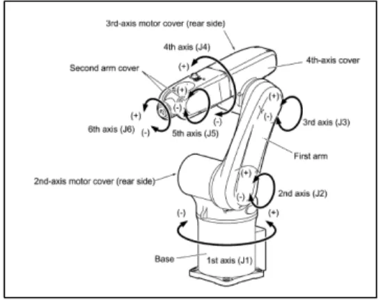
This section represents the simulation results of the position and velocity control of a eight-link robotic manipulator by the proposed adaptive control algorithm, as shown in Fig.2, and discusses the advantages of using joint controller based-on DSPs for motion control of a dual-arm robot. The adaptive scheme developed in this paper will be applied to the control of a dual-arm robot with eight axes. Fig.2 represents link coordinates of the dual-arm robot. Table Ⅰ lists values of link parameters of the robot.
그림2. 로봇의 링크 좌표계 Fig.2. Link coordinates of robot arm
Table Ⅱ lists motor parameters. Consider the dual-arm robot with the end-effector grasping a payload of mass ∆. The emulation set-up consists of a TMS320 evm DSP board and a Pentium III personal computer(PC). The TMS320 evm cardisan application development tool which is based on the TI's TMS320C80 floating-point DSP chip with 50ns instruction cycle time. The adaptive control algorithm is loaded into the DSP board, while the manipulator, the drive system, and the command generator are simulated in the host computer in C language. The communication between the PC and the DSP board is done via interrupts.
These interrupts are managed by an operating system called A shell which is an extension of Windows9x. It is assumed that drive systems are ideal, that is, the actuators are permanent magnet DC motors which provide torques proportional to actuator currents, and that the PWM inverters are able to generate the equivalent of their inputs.
In all simulations the load is assumed to be unknown. The adaptive control algorithm given in equation (10) and parameter adaptation rules (28) - (33) as are used for the motion control of robot. The parameters associated with adaptation gains are selected by hand turning and iteration as
, , ,
, , ,
, , , ,
, , ,
, , , ,
, , , , and .
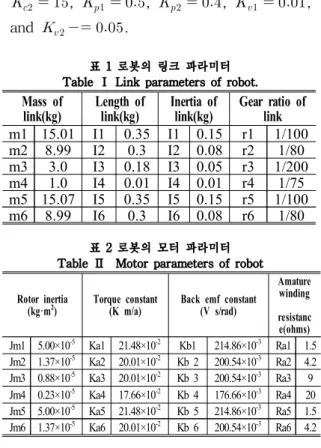
표 1 로봇의 링크 파라미터 Table Ⅰ Link parameters of robot.
Mass of link(kg)
Length of link(kg)
Inertia of link(kg)
Gear ratio of link m1 15.01 I1 0.35 I1 0.15 r1 1/100
m2 8.99 I2 0.3 I2 0.08 r2 1/80
m3 3.0 I3 0.18 I3 0.05 r3 1/200
m4 1.0 I4 0.01 I4 0.01 r4 1/75
m5 15.07 I5 0.35 I5 0.15 r5 1/100
m6 8.99 I6 0.3 I6 0.08 r6 1/80
표 2 로봇의 모터 파라미터 Table Ⅱ Motor parameters of robot
Rotor inertia (kg·m2)
Torque constant (K m/a)
Back emf constant (V s/rad)
Amature winding resistanc e(ohms) Jm1 5.00×10⁻⁵ Ka1 21.48×10⁻² Kb1 214.86×10⁻³ Ra1 1.5 Jm2 1.37×10⁻⁵ Ka2 20.01×10⁻² Kb 2 200.54×10⁻³ Ra2 4.2 Jm3 0.88×10⁻⁵ Ka3 20.01×10⁻² Kb 3 200.54×10⁻³ Ra3 9 Jm4 0.23×10⁻⁵ Ka4 17.66×10⁻² Kb 4 176.66×10⁻³ Ra4 20 Jm5 5.00×10⁻⁵ Ka5 21.48×10⁻² Kb 5 214.86×10⁻³ Ra5 1.5 Jm6 1.37×10⁻⁵ Ka6 20.01×10⁻² Kb 6 200.54×10⁻³ Ra6 4.2
It is assumed that sec,
, and , in the reference model. The sampling time is set as 0.001 sec. Simulations are performed to evaluate the position and velocity control of each joint under the condition of payload variation, inertia parameter uncertainty, and reference trajectory variation. Control performance for the reference trajectory variation is tested for four different position reference trajectories C and velocity reference trajectories M for each joint. As can be seen in Figs. 3 to 6, position reference trajectories C and velocity reference trajectory D consist of four different trajectories for joints 1, 2, 3, and 4.
The performance of DSP-based adaptive controller is evaluated in tracking errors of the position and velocity for the four joints.
The results of trajectory tracking of each joint in the different position cases are shown in Fig.'s 3∼6. Fig. 3 shows results of angular position trajectory tracking and parameter uncertainties (6%) for each joint with a 4 kg payload and parameter uncertainties (6%) for reference trajectory C.
Fig. 4 shows position trajectory tracking error for each joint with a 4 kg payload and parameter uncertainties (6%) As can be seen from these results, the DSP-based adaptive controller represents extremely good performance with very small tracking error and fast adaptation response under the payload and parameter uncertainties.
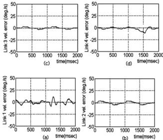
Fig. 5. shows results of angular velocity tracking at each joint with payload (4 kg), parameter uncertainties (6%), for the reference trajectory D. Fig. 6 shows results of angular velocity tracking error at each joint with payload (4 kg), parameter uncertainties (6%) for reference trajectory D. As can be seen from Fig.'s 5 and 6, the proposed adaptive controller represents good performance in the position and velocity at each joint for payload variation, inertia parameter uncertainty, and the change of reference trajectory. These simulation results illustrate that this DSP-based adaptive controller is very robust and suitable to real-time control due to its fast adaptation and simple structure.
그림 3. (a)-(d) 기준궤적C에 대한 10kg 부하하중과 10%의 관성 파라미터 불확실성을 갖는 각 관절의 위치추적성능 Fig. 3. (a)-(d) Position tracking performance of each
joint with 4kg payload and inertia parameter uncertainty (6%) for reference trajectory C.
그림 4. (a)-(d) 기준궤적C에 대한 10kg 부하하중과 10%의 관성 파라미터 불확실성을 갖는 각 관절의 위치추적오차 Fig. 4. (a)-(d) Position tracking error of each joint with
10kg payload and inertia parameter uncertainty (10%) for reference trajectory C.
그림 5. (a)-(d) 기준궤적D에 대한 10kg 부하하중과 10%의 관성 파라미터 불확실성을 갖는 각 관절의 속도추적성능 Fig. 5. (a)-(d) Velocity tracking performance of each
joint with 10kg payload and inertia parameter uncertainty (10%) for reference trajectory D.
그림 6. (a)-(d) 기준궤적D에 대한 10kg 부하하중과 10%의 관 성 파라미터 불확실성을 갖는 각 관절의 속도추적오차 Fig. 6. (a)-(d) Velocity tracking error of each joint with 10kg payload and inertia parameter uncertainty(10%) for
reference trajectory D.
The performance test of the proposed adaptive controller has been performed for the dual-arm robot at the joint space and cartesian space. At the cartesian space, it has been tested for the peg-in-hole tasks, repeating precision tasks, and trajectory tracking for B-shaped reference trajectory. At the joint space, it has been tested for the trajectory tracking of angular position and velocity for a dual-arm robot made in Samsung Electronics Company in Korea. Fig.
7 represents the experimental set-up equipment. To implement the proposed adaptive controller, we used our own developed TMS320C80 assembler software.
Also, the TMS320C80 emulator has been used in experimental set-up. At each joint of a dual-arm robot, a harmonic drive (with gear reduction ratio of 100 : 1 for joint 1 and 80 : 1 for joint 2) has been used to transfer power from the motor, which has a resolver attached to its shaft for sensing angular velocity with a resolution of 8096 (pulses/rev). Fig. 8 represents the block diagram of the interface between the PC, DSP, and robot arm.
The performance test in the joint space is performed to evaluate the position and velocity control performance of the four joints under the condition of payload variation, inertia parameter uncertainty, and change of reference trajectory.
5. Conclusions
A new robust control scheme was proposed of robotic manipulators with six joint for forging process automation. The control laws are derived from the improved Lyapunov second method. The simulation results show that the proposed controller is robust to the payload variation, inertia parameter uncertainty, and change of reference trajectory. This controller has been found to be suitable to the real-time control of robot system.
ACKNOWLEDGEMENT
This work is supported by the Kyungnam University Research Fund, 2003.
References
[1] S. Nicosia and P. Tomee, "Model Reference Adaptive Control Algorithm for Industrial Robots," Automatics, Vol. 20, No. 5, pp.
635-644, 1984.
[2] P. Tomei, "Adaptive PD Controller for Robot Manipulators," IEEE Trans. Robotics and Automation, Vol.7, No.4, Aug, 1991.
[3] R. Ortega and M.W. Spong, "Adaptive Motion Control of Rigid Robots: A Tutorial,"
Automatics, Vol. 25, pp. 877-888, 1989.
[4] A. Koivo and T. H. Guo, "Adaptive Linear Controller for Robot Manipulators." IEEE
Transactions and Automatic Control, Vol.
AC-28, pp. 162-171, 1983.
[5] H. Berghuis, R.Orbega, and H.Nijmeijer, "A Robust Adaptive Robot controller," IEEE Trans., Robotics and Automation, Vol. 9, No.
6, pp. 825-830, 1993.
[6] J. J. Craig, "Adaptive Control of Meduanical Manipulator," Addison-wesley, 1988.
[7] D. Koditschek, "Quadratic Lyapunov Functions for Mechanical Systems," Technical Report No. 8703, Yale University, New Haven, CT, 1983.
[8] T.C. Hasi, "Adaptive Control Scheme for Robot Manipulators-A Review," In Proceeding of the 1987 IEEE Conference on Robotics and Automation, San Fransisco, CA, 1986.
[9] S. Dubowsky, and D.T. DesForges, "The Application of Model Reference Adaptation Control to Robot Manipulators," ASME J. Dyn.
Syst., Meas., Contr., Vol. 101, pp. 193-200, 1979.
[10] Y.M. Yoshhiko, "Model Reference Adaptive Control for Nonlinear System with unknown Degrees," In the proceeding of American Control Conference, pp.2505-2514, Seatle, June 1995.
[11] Y.K. Choi, M.J. Chang, and Z. Bien, "An Adaptive Control Scheme for Robot Manipulators," IEEE Trans. Auto. Control., Vol. 44, No. 4, pp. 1185-1191, 1986.
[12] P.C.V. Parks, "Lyapunov Redesign of Model Reference Adaptive Control System," IEEE Trans. Auto. Control., Vol. AC-11, No. 3, pp.
362-267 , July 1966.
(접수:2016.01.05.,수정:2016.01.20, 개제확정:2016.02.05)