Casting Process Automation
A Study on Real Time Working Path Control of Vertical Type Robot System for the Forging and
Casting Process Automation
O-Deuk Lim
1, Min-Seong Kim
2*, Yang-Geun Jung
3, Jung-Suk Kang
4, Jong-Bum Won
4, Sung-Hyun Han
5<Abstract>
In this study, we describe a new approach to real-time implementation of working path control for the forging and casting manufacturing process by vertical type articulated robot system. The proposed control scheme is simple in structure, fast in computation, and useful for real-time control of factory automation based on robot system. Moreover, this scheme does not require any accurate parameter information, nor values of the uncertain parameters and payload variations. Reliability of the proposed controller is proved by simulation and experimental results for robot manipulator consisting of arm with six degrees of freedom under the variation of payloads and tracking trajectories in Cartesian space and joint space. The vertical type articulated robot manipulator with six axes made in SMEC Co., Ltd. has been used for real-time implementation test to illustrate the enhanced working path control performance for unmanned automation of the forging and casting manufacturing process.
Keywords : Forging and Casting, Vertical Articulated Robot, Working Path Control, Unmanned Automation, Payload Variations
1. Naval Shipyard
2*. Corresponding Author, M.S. Course, Graduate School Kyungnam Univ. (e-mail : [email protected]) 3. PhD. Course, Graduate School Kyungnam Univ.
4. SMEC Co., Ltd.
5. Dept. of Mechanical Engineering, Kyungnam University.
1. INTRODUCE
The convergence of the fields of robotics and automation in many industrial applications is well established. During the execution of many industrial automation tasks, the robot manipulator is often in contact with its environment (either directly or indirectly via an end-effector payload). For purely positioning tasks such as spray painting that have negligible force interaction with the environment, controlling the manipulator end-effector position results in satisfactory performance. However, in applications such as the process automation of forging or casting, the manipulator end effector will be taken an interaction forces from the environment. Furthermore, due to contact with the environment, the motion of the end effector in certain directions is restricted. In the field of robotics, this resulting motion is often referred to as constrained motion or compliant motion. This chapter focuses on the control strategies of manipulators for constrained motion. While there are many techniques that may be used to design controllers for constrained motion, a popular active compliant approach is the use of force control. The fundamental philosophy is to regulate the contact force of the environment. This is often supplemented by a position control objective that regulates the orientation and the location of the end effector to a desired configuration in its environment.[1-3]
For example, in the case of grinding applications, the motion of the manipulator arm is constrained by The grinding surface. It can easily be seen that it is vital to control not only the position of the manipulator end effector to ensure contact with the grinding surface but also the interaction forces to ensure sufficient contact force to enable grinding action.[4-6]
At recent there are mach advanced techniques that are suitable for servo control of a large class of nonlinear systems including robotic manipulators. Since the pioneering work of Dubowsky and DesForges, the interest in adaptive control of robot manipulators has been growing steadily. This growth is largely due to the fact that adaptive control theory is particularly well-suited to robotic manipulators whose dynamic model is highly complex and may contain unknown parameters. However, implementation of these algorithms generally involves intensive numerical computations.[7-9]
Current industrial approaches to the design
of robot arm control systems treat each joint
of the robot arm as a simple
servomechanism. This approach models the
time varying dynamics of a manipulator
inadequately because it neglects the motion
and configuration of the whole arm
mechanism. The changes in the parameters of
the controlled system are significant enough
to render conventional feedback control
strategies ineffective. This basic control
system enables a manipulator to perform
simple positioning tasks such as in the pick-and-place operation. However, joint controllers are severely limited in precise tracking of fast trajectories and sustaining desirable dynamic performance for variations of payload and parameter uncertainties. In many servo control applications the linear control scheme proves unsatisfactory, therefore, a need for nonlinear techniques is increasing.[10-12]
If a robot manipulator is required to draw multiple instances of one shape in the process. The end-effector position must follow a specific trajectory while ensuring that the user applies a certain amount of force on the manufacturing line. We know that if the force is too small, the drawing may not be visible; however, if the force is too large, the chalk will break. Moreover, as multiple instances of shapes are drawn, the length of the obsticles. Thus, one can appreciate complexities and intricacies of simple tasks such as drawing/writing. This example clearly illustrates the need for desired force trajectory in addition to a desired position trajectory. Another example that motivates the use of a position/force control strategy is the pick-and-place operations using grippers for glass tubes.
Clearly, if the gripper closes too tight, the glass may shatter, and if it is too lose, it is likely the glass may slip. The above examples establish the motivation for position and force control.[13-15]
In many applications, the position/force
control objectives are considerably more intertwined than in the examples discussed thus far. Consider the example of a circular diamond-tipped saw cutting a large block of metal, wherein the saw moves from one end to the other. The motion from one end to the other manifests itself as the position control objective, whereas cutting the block of metal without the saw blade binding is the force control objective. The speed of cutting (position control objective) depends on many parameters, such as geometric dimensions and material composition. For example, for a relatively softer metal such as aluminum, the saw can move safely from one end to the other much faster than in the case of a relatively harder material such as steel. It is obvious that the cutting speed would be much faster for thinner blocks of metal.[16]
To achieve control objectives such as those discussed above, the controller must be designed to regulate the dynamic behavior between the force exerted on the environment and the end effector motion.
2. MODELING
This section presents the formulation of the manipulator dynamics that facilitates the design of strategies to control robot arms.
First, the widely known joint-space model is
presented. Next, we define some notation for
the contact forces (sometimes referred to as
interactive forces) exerted by the manipulator on the environment by employing a coordinate transformation.[17-18]
2.1 Joint-Space Model
The dynamics of motion for an n-link robotic manipulator are constructed in the Euler-Lagrange form as follows:
(1)
Where
(2)
∈
×denotes the inertia matrix,
∈
×contains the centripetal and Coriolis terms, ∈
contains the static (Coulomb) and dynamic (e.g., viscous) friction terms, ∈
is the gravity vector,
∈
represents the joint-space end- effector forces exerted on the environment by
the end-effector, ∈
represents the joint-space variable vector, and ∈
is the torque input vector.[18-19]
2.2 Joint-Space Model
In order to facilitate the design of force controllers, the forces are commonly transformed into the task-space via a Jacobian matrix by using a coordinate transformation. [20-21] Note that this Jacobian matrix is defined in terms of the task-space coordinate system and dependent on the robot application. Specifically, depending on the type of application, the axes of force control and motion may vary and are captured by the definition of the Jacobian.[22] Toward formulating the task- space dynamics, we define a task-space vector ∈
as follows:
(3)
Where is obtained from the manipulator kinematics and the joint and task-space relationships. The derivative of the task-space vector is defined as follows :
(4)
Where the task-space jacobian matrix
∈
×is defined as [23-24]
(5)
Fig.1 Link coordinates of robot manipulator
with 6-D.O.F
With being the identity matrix, being the zero matrix, and the transformation matrix is used to convert joint velocities to derivatives of roll, pitch, and yaw angles associated with end-effector orientation.[22] It should be noted that the joint-space representation of the force exerted on the environment can be rewritten as
(6)
Where ∈
denotes the vector of forces and torques exerted on the environment in task-space.[23]
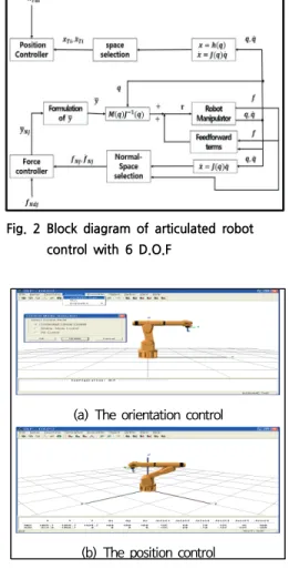
3. CONTROLLER DESIGN
An important disadvantage of the stiffness controller discussed in the previous section is that the desired manipulator position and the desired force exerted on the environment are constants. That is, the controller is restricted to a constant set point regulation objective.
In applications such as polishing and deburring, the end effector must track a prescribed path while tracking some desired force trajectory on the environment. In such a scenario, the stiffness controller will not achieve satisfactory results.[23-24]
To that end, another approach that simultaneously achieves position and force tracking objectives is used. The hybrid position/force controller developed in decouples the position and force control problems into
subtasks via a task-space formulation. This formulation is critical on determining the directions in which force or position should be controlled. Once these subtasks are identified, separate position and n-link manipulator and then discuss this control strategy with respect to the 6-DOF Cartesian manipulator shown in Fig. 1.
The following hybrid position/force controller first uses feedback-linearization to globally linearize the robot manipulator dynamics and then employs linear controllers to track the desired position and force trajectories. To that end, by using the task-space transformation of Equation (3) to decompose the normal and tangential surface motions and after some mathematical manipulation, the robot dynamics can be expressed as
(7)
Based on the structure of Equation (7) and the control objectives, a feedback-linearizing controller for the above system can be constructed as follows:
(8)
Where ∈
denotes the linear position
and force control strategies. Note that from
Equation (7) and Equation (8), we have
(9)
Given that the system dynamics in Equation (9) have been decoupled in the task-space into tangential and normal components denotes by subscripts T and N, respectively, we can design separate position and force control algorithms.[25]
The tangential task-space components of
can be represented as follows:
(10)
Where
denotes the th linear tangential task-space position controller. The corresponding tangential task-space tracking error is defined as follows:
(11)
Where
represents the desired position trajectory. Based on the controller objective and the structure of Equation (11), we can design the following linear algorithm:
(12)
where
and
are the th positive control gains. After substituting this controller defined in Equation (12) into Equation (10), we obtain the following closed-loop dynamics as follow:
( 13)
Given that
and
are positive, an asymptotic position tracking result is obtained as follow:
lim
→
(14)
The normal task-space components of
can be represented as follows:
(15)
Where
denotes the th linear normal task-space force controller. The corresponding normal task-space tracking error is defined as follows:
(16)
Where the environment is modeled as a spring,
denotes the th component of the environmental stiffness, and
represents the static location of the environment in the normal direction. The force dynamics can be formulated by taking the second time derivative of Equation (16) as follows:
(17)
Which relates the acceleration in the
normal direction to the second time
derivative of the force. To facilitate the construction of a linear controller, we define the following force tracking error as follow:
(18)
Where
denotes the th of the desired force trajectory in the normal direction. A linear controller that achieves the force tracking control objective is defined as follow:
(19)
Where
and
are th positive control gains. After substituting the controller into Equation (17), we obtain the following closed-loop dynamics equation as follows:
(20)
From equation (20), asymptotic force tracking is defined as follows:
lim
→∞