ORIGINAL ARTICLE
Filling in Water Temperature Data of Aquatic Environments using a Pre-constructed Relationship
Khil-Ha Lee*
Department of Civil Engineering, Daegu University, Gyeongsan 38453, Korea
Abstract
In this study a method for filling in missing data of river water temperature using a pre-constructed mathematical relationship between air and water temperatures is presented. A regression between water temperatures at individual stations and ambient air temperatures at nearby weather stations can provide a practical method for representing missing water temperature data for an entire region. Air and water temperature data that were collected from two test sites (one coastal and, one inland) were individually fitted to a nonlinear regression model. To consider seasonal hysteresis effects, separate functions were fitted to the data in the rising and falling limbs. A single-criterion, multi-parameter optimization technique was used to determine the optimal parameter sets. This method minimizes the differences between the time series of the measured and estimated data. The constructed air-water temperature relationship was subsequently applied to represent missing water temperature data. It was found that the RMSEs(MBEs) were in the range of 1.843―1.976oC(-0.329―0.201oC) and the coefficient of determination were in the range of 0.92―0.96. The results demonstrate that the predicted water temperatures using the regression equations were reasonably accurate.
Key words : Missing data, Logistic function, Optimization, Water temperature
1. Introduction1)
In most studies related to hydrologic research, missing data occur for several reasons, such as malfunctioning equipment and data collection and/or recording mechanisms, data entry errors, sensor failure, sensor replacement, and miscalibration.
Missing data has the potential to substantially skew results (Schafer and Graham, 2002; Cole, 2008).
Previous work has suggested that all researchers examine their data for missing data and address missing data in the most appropriate and desirable way to ensure high-quality results (Rubin, 1976;
Cole, 2008; Osborne, 2013).
The topic of missing data has gained considerable attention in the last decade. However, several important misunderstandings remain regarding the problems that missing data can generate and acceptable solutions for addressing these data (Little and Rubin, 1987).
Water temperature affects the Dissolved Oxygen (DO) levels in estuarine and river habitats because saturated DO is lowest at higher water temperatures, which often occur during summer (Lee and Lwiza, 2007). Hence, water temperature is an important
Received 6 September 2017; Revised 28 September, 2017;
Accepted 10 October, 2017
*Corresponding author: Khil-Ha Lee, Department of Civil Engineering, Daegu University, Gyeongsan 38453, Korea
Phone: +82-53-850-6522 E-mail: [email protected]
ⓒ The Korean Environmental Sciences Society. All rights reserved.
This is an Open-Access article distributed under the terms of the Creative Commons Attribution Non-Commercial License (http://
creativecommons.org/licenses/by-nc/3.0) which permits unrestricted non-commercial use, distribution, and reproduction in any medium, provided the original work is properly cited.
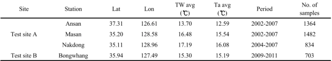
Site Station Lat Lon TW avg ( )
Ta avg
( ) Period No. of
samples Test site A
Ansan 37.31 126.61 13.70 12.59 2002-2007 1364
Masan 35.20 128.58 16.48 15.54 2002-2007 1482
Nakdong 35.11 128.96 17.19 16.08 2004-2007 834
Test site B Bongwhang 35.94 127.49 15.30 15.19 2009-2011 703
Table 1. Summary of observed stations used for this study factor for the quality of water resources and aquatic environment. Moreover, a change in water temperature results in a change in the water resources quality, especially the DO levels, which change the aquatic biota (Stefan and Sinokot, 1993; Pilgrim and Stefan, 1995; Mohseni et al., 1998; Mohseni et al., 1999;
Mohseni and Stefan, 1999; Mohseni et al, 2002;
Struyf et al., 2004; Morril et al., 2005). The temporal trend in water temperatures varies according to the temporal variations in air temperature, which exhibits both seasonal and diurnal patterns. The effects of air temperature on water temperature have been previously reported; some efforts have been made to formulate air-water temperature relationships (Mohseni et al., 1998; Mohseni et al., 1999; Mohseni and Stefan, 1999; Mohseni et al., 2002; Morril et al., 2005). Thus, a regression curve between water temperatures measured at individual stations and ambient air temperatures from nearby weather stations may provide a practical method to fill missing data. A time lag is often involved due to the delayed response of the water temperature due to the thermal inertia of water; however, a time lag is not necessary when using weekly averaged data (Stefan and Preud’ homme, 1993; Mohseni and Stefan, 1999). This study examines the air-water temperature relationship on the basis of a logistic function in the Korean aquatic environment. The study assumes that air temperatures are related to water temperatures in order to represent the missing data. The air-water temperature data collected from four focused sites are individually fitted to a nonlinear regression model.
Two sites are exposed to seasonal hysteresis; separate functions are fitted to the data in the rising and falling limbs to consider the seasonal hysteresis at this site.
Once a relationship between air-water temperatures is constructed from recordings, the relationship is subsequently used to address the missing water temperature data. The study uses a single-criterion, multi-parameter optimization scheme to obtain an optimal parameter set in constructing the air-water relationship.
2. Study region and data
The Korea Institute of Ocean Science and Technology (KIOST) has focused on collecting air and water temperature data, meteorological data, and data regarding water quality at three estuarine sites:
Ansan, Masan, and Nakdong (hereafter called test site A). Table 1 presents the study location and the weather data, which was averaged over the study period. The Ansan site, which has three individual stations, is situated within a closed territory that is surrounded by a sea wall; this site occasionally has contact with the ocean when the gate is open. The Masan site, which has two individual stations, is partially exposed to the ocean, whereas the Nakdong site is completely enclosed by a sea wall with no contact with the ocean because the sea wall prevents ocean intrusion.
The meteorological data used in this study were from the period 2002-2007, consisting of carefully screened daily values. The air and water temperatures,
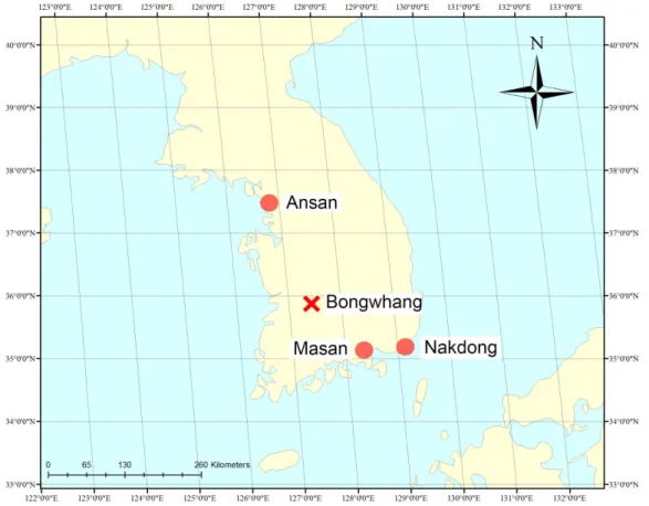
Fig. 1. Test site A (circles) and B (cross): Test site A (Ansan, Masan, and Nakdong) are in coastal zones, which represent both river and ocean systems. Test site B is in inland zones.
which were simultaneously collected by the KORDI at the same location, were obtained using a CTD sensor, OS-316. The water temperatures were measured at approximately 1 m below the water surface, while the air temperatures were measures at approximately 2 m above the water surface. The measured data were averaged over 5-min intervals in this study. Fig. 1 (circles) show the first test sites (coastal with three stations). The collected data from each meteorological station were previously checked for integrity, quality, and reasonableness according to different tests (Meek and Hatfield, 1994; Shafer et al., 2000; Schafer and Graham, 2002). Any observation that was beyond the allowable range was eliminated.
The Korea peninsula has a moderate climate
characterized by distinct wet and dry seasons. The dry season coincides with a predominant northwesterly wind, which typically occurs from October to March.
The wet season results from a predominant southeasterly wind, which transports moisture-laden air from the Pacific Ocean and lasts from May to October; 70% of the annual precipitation falls during this season.
Moreover, July and August are usually the wettest months.
All sites exhibit typical daily and seasonal temper -ature variations. The seasonal maximum temperature typically occurs between May and October, while the minimum temperature occurs between November and April. Estuarine sites generally exhibit smaller temperature variations; the Diurnal Temperature
Range (DTR) is approximately 7 .
A second location was tested to demonstrate the practicality and the universal applicability of the proposed method. While the first test site was located at a coastal area, an inland area was selected for the second test site (Fig. 1; cross). The water temperature data were provided by the National Institute of Environmental Research (NIER), Bongwhang, Korea (hereafter called test site B); the corresponding air data used in this study were collected by the Korea Meteorological Administration (KMA). The data used for this study were recorded between January 2009 and December 2011 and consist of carefully screened daily values. The mean and standard deviation of the water temperature at the Bongwhang station are approximately 15.3 and 7.36 , respectively.
Several factors may affect the relationship between air and water temperatures, including human use, current temperature, the air-water interface, and heat exchange (Stefan and Sinokot, 1993; Pilgrim and Stefan, 1995; Mohseni et al., 1998; Mohseni et al., 1999; Mohseni and Stefan, 1999; Mohseni et al., 2002; Morril et al., 2005). In the estuarine environment, such as the test sites in this study, an additional tidal effect from the ocean may occur with seasonal implications. There is no reservoir release upstream from the gauging station; however, some interaction with the groundwater inflow to the gauging station does occur.
3. Mathematical models
Regression approaches are advantageous because they often require only one climate variable, air temperature. However, some studies have concluded that a linear regression function is not sufficient for determining year-round water temperatures because the air-water temperature relationship does not typically remain linear for the highest and lowest air temperatures (Pilgrim and Stefan, 1995; Mohseni et
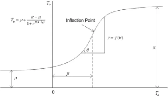
al., 1998; Mohseni and Stefan, 1999). Alternatively, a nonlinear curve, called a logistic function, has been suggested for describing the nonlinear nature of the air-water temperature relationship. A logistic function is a common sigmoid function that is primarily used for population growth models (Richard, 1959; Pella and Tomlinson, 1969). Logistic functions are good models for biological population growth in species and marketing for the sales of new products (Lei and Zhang, 2004). The initial stage of growth follows an exponential curve before the growth slows down as saturation begins to occur. At the maturity stage, growth eventually stops. Every logistic curve has a single inflection point that separates the curve into two equal regions of opposite concavity (Lei and Zhang, 2004). This inflection point is called the point of diminishing returns (Richard, 1959; Pella and Tomlinson, 1969; Lei and Zhang, 2004); the derivative of the logistic function attains its maximum at the inflection point. The general form of a logistic function is as follows:
( )
1 Ta
w e
T (1)
where Tw is the air temperature-dependent water temperature and Ta is the air temperature over the period of interest. Equation (1) has four parameters, (i.e., is the upper asymptote, is the time of maximum growth; is the growth rate, and ) is the lower asymptote. The parameters , , , and represent the maximum water temperature, the air temperature at the inflection point, a function of the largest slope in the Tw function with respect to Ta, and the minimum water temperature, respectively. Hence
should be greater than . Fig. 2 presents a schematic plot for equation (1). is about mid-point of maximum and minimum air temperature., and maximum and minimum air temperatures could be set for constraint. The slope in the Tw is not steep and
is usually less than 1~2, and ≦ ≦ was used for this study.
One of the most important issues in this modeling approach is to determine the model parameters, which strongly affect the accuracy of the model (Duan et al., 1993, 1994; Chau, 2007).
Fig. 2. A Schematic plot for the logistic function.
A single-criterion optimization technique was used to minimize the differences between the time series of measured and modeled water temperatures. Moreover, the feasibility of estimating the four parameters was also investigated. In general, a numerical model may have n parameters (in this case, the parameters describe the maximum water temperature, the minimum water temperature, the air-water temperature slope, and the air temperature at the inflection point) to be calibrated using m observations (in this case, the time series of measured water temperatures). The distance between the m model-simulated responses and the m observations is defined by an objective function (O), such as the Root-Mean-Square Error (RMSE), between the modeled responses and observations.
The goal of the model calibration step is to determine the preferred value for the n parameters within the feasible set of parameters that minimize O.
The Shuffled Complex Evolution algorithm (SCE, Duan et al., 1993, 1994) is a general-purpose global optimization method designed to handle many of the response problems encountered in the calibration of
nonlinear simulation models. The algorithm randomly samples the feasible parameter space, which is prescribed to encompass only reasonable values in this study, to obtain a population of points. The population is subsequently partitioned into several
“complexes”. Each complex evolves independently in a manner based on the downhill simplex algorithm (Nelder and Mead, 1965). Readers are referred to Duan et al. (1993, 1994) for more details on the numerical algorithm.
4. Results
The data at each test site were divided into two groups. The first group was used for calibration, while the second group was used for validation (partially selected data). For the second group, approximately 20-30 points were randomly not included in the procedure to represent missing data in both the wet and dry seasons at each station. A relationship between air and water temperatures must be constructed before filling in the missing data.
Therefore, the first group of data was used to determine the preferred parameter set using the single-criterion optimization technique that was discussed in the previous section. Moreover, patterns must be identified; the existence of a hysteresis must also be verified because a hysteresis may be involved in the air-water temperature relationship (Webb and Nobilis, 1997; Mohseni et al., 1998). To verify the existence of a hysteresis at each site, the rising and falling limbs were distinguished from each other. To separate the annual cycle into the rising and falling limbs, the week associated with the minimum mean weekly air temperature was regarded as the starting point of the rising limb (which also corresponds to the ending point of the falling limb), while the week associated with the maximum mean weekly air temperature was regarded as the ending point of the rising limb (which also corresponds to the starting
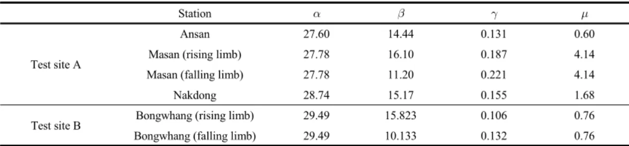
Station
Test site A
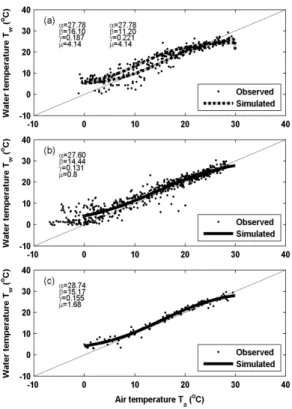
Ansan 27.60 14.44 0.131 0.60
Masan (rising limb) 27.78 16.10 0.187 4.14
Masan (falling limb) 27.78 11.20 0.221 4.14
Nakdong 28.74 15.17 0.155 1.68
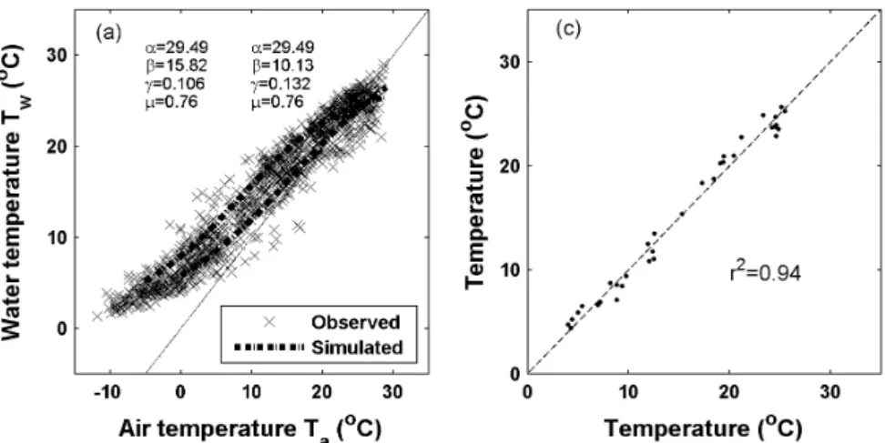
Test site B Bongwhang (rising limb) 29.49 15.823 0.106 0.76
Bongwhang (falling limb) 29.49 10.133 0.132 0.76
Table 2. Preferred logistic function parameter sets for each site. The parameter sets are optimized using the SCE scheme
point of the falling limb).
4.1. Validation of test site A
After checking for the existence of a hysteresis at the three locations, the Masan site was found to exhibit a noticeable hysteresis (Fig. 3). Table 2 presents the preferred parameter set (i.e., , , , and
) for each site. To quantify the efficiency of the fit, the Nash-Sutcliffe Coefficient of efficiency (NSC) (Nash and Sutcliffe, 1970) was used. The normal distribution of the error structure was assumed to determine the confidence intervals of the regression model. The results show that the NSCs for the Ansan and Nakdong sites are 0.917 and 0.967, respectively, for the calibration process. All the sites show some local biases. The RMSEs(MBEs) for the Ansan and Nakdong sites are 1.826 (-0.227 ) and 1.388 (0.188 ), respectively. For the Masan site, the NSCs for the rising and falling limbs are 0.901 and 0.929, respectively, while the RMSEs(MBEs) for the rising and falling limbs are 1.918 (-0.136 ) and 1.765 (-0.125 ), respectively. There is an indication that the falling limb is slightly better fitted than the rising limb. The estimated water temperatures using the logistic air-water temperature relationship exhibit reasonable accuracy at each site.
The second group is used to examine the accuracy and performance of the suggested method for the validation process. Comparisons between measured and estimated water temperatures using equation (1) at the three stations are presented in Fig. 4-5. The
RMSEs(MBEs) for the Ansan and Nakdong sites are 1.962 (-0.220 ) and 1.425 (-0.132 ), respectively.
For the Masan site, the RMSEs(MBEs) for the rising and falling limbs are 1.976 (-0.329 ) and 1.863 (-0.308 ), respectively. The coefficients of determination are 0.92, 0.93, and 0.96 for the Ansan, Masan, and Nakdong stations, respectively.
Fig. 3. Weekly mean water temperatures in the Masan station during the year of 2005. Separate warming and cooling season track account for hysteresis in the dataset. The numbers indicate the week of the year.
4.2. Validation of test site B
Test site B also exhibits a hysteresis; the preferred parameter sets for each site are presented in Table 2.
The NSCs for the rising and falling limbs are 0.925 and 0.940, respectively, while the RMSEs for the rising and falling limbs are 1.924 and 1.717, respectively. The general trend is similar to the trend observed at test site A. Using the same method described for test site A, the second group is used to
Fig. 4. Fitted water temperatures against the observed water temperatures. The preferred parameter set are shown in Fig. 4(a-c): a) the Masan site, b) the Ansan site, and c) the Nakdong site. The values on the left in Fig. 5(a) are for the rising limb, while the values on the right in Fig. 5(a) are for the falling limb.
Fig. 5. A scatter plot of estimated versus measured missing water temperature data using the logistic air-water temperature relationship; (a) Ansan station, (b) Masan station, and (c) Nakdong station.
examine the accuracy and performance of the suggested method for the validation process.
Comparisons between the measured water temperatures and those estimated using equation (1) at site B are presented in Fig. 6(b). The RMSE(MBE) and the coefficient of determination are 1.843 (0.201 ) and 0.94, respectively, for the validation station.
As a whole, the RMSEs and MBEs are within acceptable accuracy, and the coefficient of determination is excellent with over 0.9. Very large errors are unlikely to occur in estimation. In general, the logistic air-water temperature relationship provides a reasonable method for handling missing water temperature data.
5. Summary and conclusions
Air and water temperature data collected from three focused sites are individually fitted to a nonlinear regression model to handle missing data.
First, a single-criterion optimization technique is used to determine the four parameters of the logistic function, which are used to adequately reflect the characteristics of local climate and to minimize the differences between the measured and modeled water temperature time series. Subsequently, the calibrated model is used to fill in missing water temperature data. Finally, the estimated water temperatures using the logistic air-water temperature relationship are compared to those measured in the field. The primary
Fig. 6. (a) Fitted water temperatures against the observed water temperatures. (b) A scatter plot of estimated versus measured missing water temperature data using the logistic air-water temperature relationship.
conclusions are as follows:
The SCE optimization scheme provides reasonable estimates of the logistic function parameters for the air-water temperature relationship.
The Masan site and test site B exhibit a noticeable seasonal hysteresis; therefore, separate functions must be fitted.
The RMSEs(MBEs) for the Ansan, Nakdong, and Bongwhang sites are 1.962 (-0.220 ), 1.425 (-0.132 ), and 1.843 (0.201 ), respectively. The RMSEs(MBEs) of the rising and falling limbs for the Masan station are 1.976 (-0.329 ) and 1.863 (-0.308 ), respectively.
There are some local biases but the estimated water temperatures using the logistic air-water relationship are shown to be reasonably accurate for representing missing water temperature data.
The results from this study show that the logistic air-water temperature relationship is very effective for predicting water temperatures with respect to ambient air temperatures in an aquatic environment.
This study provides a simple method to handle missing water temperature data that may be difficult to address in practice. Unfortunately very limited field measurement may limit the degree of validation
of the suggested model. To collect a reliable database from more regions and conduct general validation would be desirable and beneficial.
Acknowledgements
This research was financially supported by the Research Program #20160156 at Daegu University.
REFERENCES
Chau, K. W., 2007, A Split-step particle swarm optimization algorithgm in river stage forecasting, Journal of Hydrology, 346(3-4), 131-135.
Cole, J. C., 2008, How to deal with missing data, In:
Osborne, J. W. (ed.), Best practices in quantitative method, Thousand Oaks, C.A. Sage, 214-238.
Duan, Q. Y., Gupta, V. K., Sorooshian, S., 1993, Shuffled complex evolution approach for effective and efficient global minimization, Journal of Optimization Theory and Applications, 76, 501-521.
Duan, Q. Y., Sorooshian, S., Gupta, V. K., 1994, Optimal use of the SCE-UA global optimization method for calibrating watershed models, Journal of Hydrology, 158, 265-284.
Lee, Y. J., Lwiza, K. M. M., 2007, Characteristics of bottom dissolved oxygen in Long Island Sound, New York, Estuarine, Coastal and Shelf Science, 76,
187-200.
Lei, Y. C., Zhang, S. Y., 2004, Features and partial derivatives of Bertalanffy-Richards growth model in forestry, Nonlinear Analysis: Modeling and Control, 9(1), 65-73.
Little, R. J. A., Rubin, D. B., 1987, Statistical analysis with missing data, John Wiley & Sons, New York.
Meek, D. W., Hatfield, J. L., 1994, Data quality checking for single station meteorological databases, Agricultural and Forest Meteorology, 69, 85-109.
Mohseni, O., Ericson, T. R., Stefan, H., 1999, Sensitivity of stream temperature in the United States to air temperature projected under a global warming scenario, Water Resources Research, 35(12), 3723- 3733.
Mohseni, O., Ericson, T. R., Stefan, H., 2002, Upper bounds for stream temperature in the contiguous United States, Journal of Environmental Engineering, 128(1), 4-11.
Mohseni, O., Stefan, H., 1999, Stream temperature/air temperature relationship: A Physical interpretation, Journal of Hydrology, 218, 128-141.
Mohseni, O., Stefan, H., Ericson, T. R., 1998, A Nonlinear regression model for weekly stream temperature, Water Resources Research, 34(10), 2685-2692.
Morril, J. C., Bales, R. C., Conklin, M. H., 2005, Estimating stream temperature from air temperature:
Implications for future water quality, Journal of Environmental Engineering, 131(1), 139-146.
Nash, J. E., Sutcliffe, J. V., 1970, River flow forecasting through conceptual models, I-A Discussion of principles, Journal of Hydrology, 10, 282-290.
Nelder, J. A., Mead, R. A., 1965, A Simplex method for function minimization, Computer Journal, 7, 308-313.
Osborne, J. W., 2013, Best practices in data cleaning: A Complete guide to everything you need to do before
and after collecting your data, Sage Publication: USA.
Pella, J. J. S., Tomlinson, P. K., 1969, A Generalized stock-production model, Bull. IATTC., 13(3), 421-496.
Pilgrim, J. M., Stefan, H. G., 1995, Correlation of Minnesota stream water temperatures with air temperatures, Project. Rep. 382. St Anthony Falls Laboratory, University of Minnesota, Minneapolis.
Richards, F. J., 1959, A Flexible growth function for empirical use, Journal Experimental Botany, 10(2), 290-300.
Rubin, D., 1976, Inference and missing data, Biometrika, 63(3), 581-592.
Schafer, J. L., Graham, J. W., 2002, Missing data: Our view of the state of the art, Psychological Methods, 7, 147-177.
Shafer, M. A., Fiebrich, C. A., Arndt, D. S., 2000, Quality assurance procedures in the Oklahoma Mesonetwork, Journal of Atmospheric and Oceanic Technology, 17(4), 474-494.
Stefan, H. G., Preud’ homme, E. B., 1993, Stream temperature estimation from air Temperature, Water Resources Research, 29(1), 27-45.
Stefan, H. G., Sinokrot, B. A., 1993, Projected global climate change impact on water temperatures in five north central U.S. streams, Climate Change, 24(4), 353-381.
Struyf, E., Damme, S. V., Meire, P., 2004, Possible effects of climate change on estuarine nutrient fluxes: A Case study in the highly nutrified Schelde estuary (Belgium, The Netherland), Estuarine Coastal and Shelf Science, 60, 649-661.
Webb, B. W., Nobilis, F., 1997, Long term perspective on the nature of the air-water temperature relationship: A Case study, Hydrological Processes, 11, 137-147.