개인고속이동 시스템의 차량제어용 속도 프로파일 생성과 속도 추종을 위한 제어 시스템 설계
Generation of Speed Profile for the Control of a Personal Rapid Transit Vehicle and the Design of the Control System for the Speed
Tracking
이준호(1) 신경호(2) 이재호(3) 김용규(4)
Jun-Ho Lee, Kyung-Ho Shin, Jea-Ho Lee, Yong-Kyu Kim
--- ABSTRACT
본 논문에서는 개인고속이동(PRT: Personal Rapid Transit)시스템에서 차량의 속도를 제어하기 위해서 필요한 속도 프로파 일의 생성과, 생성된 속도 프로파일의 추종 특성을 관찰하기 위한 제어 시스템의 구축에 관해서 다룬다. 제어 시스템을 구 축하기 위해서 Labview Real Time Module과 Matlab/Simulink 를 채용한다. 제어기준신호인 속도 프로파일은 간단한 선형 방정식을 이용해서 생성할 수 있으며 방정식에 포함되어 있는 변수들에 대한 정보를 얻기 위해서 가상의 선행차량으로부터 feedback되는 차량의 상태정보를 이용한다. 간단한 모의시험을 통해서 속도 프로파일 추종특성의 평가를 위한 제안된 제어 시스템의 효용성을 보인다.
---
1. Introduction
A fundamental concept of the personal rapid transit system has been introduced in the Individualized Automated Transit in the City in 1964. From the late 1960's Aerospace Corporation, involved in US government, began the system analysis and the development of the technical theory. Based on the historical back ground West Virginia Univ. employed the PRT system in the early 1970's as a transportation means connecting downtown of the city of Morgantown and the University campus. This transit system is still in operation. In other systems, Cabintaxi of Germany, Ultra of UK, Taxi 2000 of USA have been trying to commercialize the PRT system from the early 1980's. In case of Korea since the PRT system has been introduced in the early 1990's a great effort has been invested for the development of the system and commercialization [1]. Since the fundamental concept of the PRT system is to make it possible for the vehicle to go to its final destination without stopping, with very short headway, in maximum speed 40-50[km/h], with 4-5 passengers per vehicle, the vehicle control algorithm plays a very important role to avoid the impact between the vehicles. The vehicle control module is basically made of the state information of the preceding and the rear vehicles, vehicle dynamics, and the speed profile that the rear vehicle should be tracked. The speed profile is produced by the central control computer or by the vehicle on-board computer based on the state information of the preceding and the rear vehicles [2],[3],[4],[5].
---
(1) 책임저자, 정회원, 한국철도기술연구원, 전기신호연구본부 E-mail : [email protected] TEL : (031)460-5040 FAX : (031)460-5449
(2) 한국철도기술연구원, 전기신호연구본부 (3) 한국철도기술연구원, 전기신호연구본부 (4) 한국철도기술연구원, 전기신호연구본부
The dynamics of the conventional rail trains have been studied for a long time and can be described by established equations. Many simulation programs already exist and are used by the academia and the industry [6]. On the other hand the vehicle control and the simulation programs for the PRT system are still in the developing phase, not a mature commercial technology.
In this paper we deal with a novel method to construct a control system using Labview Simulation Interface Toolkit and Matlab/Simulink combined system which is composed of modulized blocks. The vehicle equation of motion is expressed by using the simple linear DC motor. In order to guarantee the tracking performance we employ a proportional and differentiation compensator. It should be noted that we select the linear DC motor for the vehicle traction to simplify the modeling of the vehicle dynamics, however a linear induction motor, a linear synchronous motor or a rotational motor can be employed for the vehicle traction based on the design scheme of the traction system. The speed profile is induced by using a simple quadratic equation. In this paper we assume that the maximum vehicle speed is 40-50[km/h] and we consider the voltage control of the linear DC motor for the brake system, which means that we do not consider frictional brake system.
First we show the equation of motion for the vehicle and the inducement of the quadratic equation to derive the speed profile, and then the construction of the control system is introduced. Finally the simulation results present that the proposed control system is effective to show the tracking performance.
2. Motion of Equation
Fig. 1 shows the simple schematic diagram of the vehicle traction. Linear DC motor is employed as the
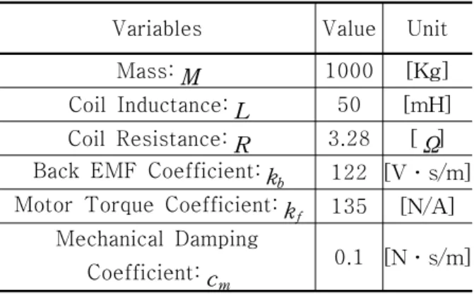
traction system. Table 1. shows the each parameters for the system model shown in Fig. 1. The equation of motion of the linear DC motor is
M ẍ+cm ẋ=F=kfi (1) where F is the traction force produced by the linear motor, i is the coil current to control the traction force, x is the vehicle displacement in longitudinal direction .
The voltage equation of the coil is
Table 1. Parameters to calculate headway
Variables Value Unit
Mass: M 1000 [Kg]
Coil Inductance: L 50 [mH]
Coil Resistance: R 3.28 [ Ω]
Back EMF Coefficient: kb 122 [V․s/m]
Motor Torque Coefficient: kf 135 [N/A]
Mechanical Damping Coefficient: cm
0.1 [N․s/m]
Fig. 1 Schematic diagram of the vehicle traction
E=Ri+Ldi
dt+Eb (2) where E is the coil voltage, Eb is the back electromotive force(emf) which is expressed such as
Eb=kbẋ (3) Equation (1), (2) and (3) yield the state space model that is
ꀎ ꀚ
︳︳
︳︳ ꀏ ꀛ
︳︳
︳︳ ẋ
ẍ
i̇
= ꀎ
ꀚ
︳︳
︳︳
︳︳
︳︳
︳︳
︳︳
︳
ꀏ
ꀛ
︳︳
︳︳
︳︳
︳︳
︳︳
︳︳
︳
0 1 0
0 -cm M
kf M 0 -kb
L -R
L ꀎ ꀚ
︳︳
︳ ꀏ ꀛ
︳︳
︳ x ẋ
i +
ꀎ
ꀚ
︳︳
︳︳
︳︳
︳ ꀏ
ꀛ
︳︳
︳︳
︳︳
︳ 0 0 1 L
E (4)
In equation (1) we do not consider the resistance force acting on the vehicle. In fact for the conventional rail train system train motion equation is described such as:
Mẍ = F-Frr-Fra-G-C (5) where Frr is the rolling and bearing friction resistance, Fra is the aerodynamic resistance, G is the grade resistance, C is the curvature resistance. Equation (5) means that the acceleration force of a train is the traction force minus the total resistance.
In this paper we ignore the rolling and bearing friction force for the traction system modeling because the traction system is the linear DC motor. Aerodynamic resistance, grade resistance, and the curvature resistance are also ignored for the simplification of the mathematical model of the traction system because the development of the accurate mathematical model is out of scope of this paper.
3. Speed Profile
In order to produce a speed profile of a vehicle, the relation of the speed between the two vehicles should be considered. As see in Fig. 2 if vehicle A reduces the vehicle speed vehicle B should also reduce the speed with the safety distance ds.
Fig 2. Distance between vehicles
In this case the initial speed of the vehicle B, vci, should be reduced to the final speed of the vehicle B, vcf, with a deceleration, a, to maintain the safety distance. Thus if the deceleration is constant the speed of the vehicle B is
vB =⌠⌡
tf
t0
-adt
=-atf+at0
=at0-vcf
(6)
where t0 is the initial time that the brake of the vehicle B is activated, tf is the final time to be reached
to the final speed. The integration of the velocity yields the moving distance of the vehicle from t0 to tf such as:
dB =⌠⌡
tf
t0
vBdt
=⌠⌡
tf
t0
(at-vcf)dt
=1
2aΔt2-vcfΔt
(7)
where Δt =tf- t0. If the distance Db that the vehicle can move is limited by the rail block system like the conventional train system or by the brick wall speed control system which has a non-block system, we can know the distance Db from the system specifications. Normally in the conventional rail train control system Db is the one block distance and in the non-block system Db is the distance which satisfies the brick wall condition. From this conditions the instantaneous position of the vehicle can be induced like this:
dBp=Db-( 1
2aΔt2-vcfΔt) (8) From eq. (8) we can get the following equation which expresses the relation between the vehicle speed and the vehicle position:
Db-dBp = 1
2aΔt2-vcfΔt
= 1
2a
(
vB+va cf)
2-vcf(
vB+va cf)
= v2B-v2cf 2a
(9)
Eq. (9) yields
vB= 2a(Db-dBp)+v2cf (10) Equation (10) means that if there are the information for the final speed to be reached, the instantaneous vehicle position, the block distance or the brick wall safety distance, and the deceleration, then it is easy to calculate the vehicle speed. In reality the vehicle speed vB is a function of time and the speed versus time indicates the vehicle speed profile, corresponding to either the speed code received from the track signaling system or the speed command set by the driver during the operation like in the conventional ATC(Automatic Train Control) system. If the train control system does not have the ATO(Automatic Train Operation) function the command speed which is set in every block should be tracked manually by the operator. Since the PRT system has very short headway and the vehicle is operated without a driver AVO(Automatic Vehicle Operation) function plays an important role in the vehicle control system. In this paper we employ a PD (Proportional and Differentiation) controller to implement the AVO function
4. Synthesis of the Control System
Fig. 3 shows the block diagram of the proposed control system. In this model the value of the input parameters, the state information of the vehicles, are decided for the initial conditions, and then the creation of the speed profile block makes an output of the speed based on the input state information. The produced speed which is the function of the moving distance of the
following vehicle is used as the reference speed in the AVO module to make the control command for the LDM. In AVO module it is possible that several different kinds of controllers can be used to control LDM through the feedback of the vehicle speed.
5. Simulations
A combined system which has Matlab/Simulink and Labview Simulation Interface Toolkit is used to simulate the algorithm that derives the speed profile and the AVO function. Matlab/Simulink is well known software to control engineers and Labview Simulation Interface Toolkit that allows the development and the test of the control system using models developed in the Simulink simulation environment. The Simulation Interface Toolkit(SIT) including the SIT server provides a way to create a Labview user interface that we use to interact with a Simulink model by way of the TCP/IP communication port. Thus using the SIT Connection Manager dialog box of Labview, we can specify the relationship between the Labview controls and indicators of the front panel and the Simulink parameters and sink blocks. Once we configure the relations between the Simulink and the Labview, the Simulation Interface Toolkit automatically generates the block diagram code necessary to establish the relationships between the Labview VI(Virtual Instruments) and the Simulink model.
There are several advantages in this method compared to the conventional simulation method using a tool like Simulink only.
1. Easy gain tuning in real time 2. Easy data acquisition
3. Easy debugging by monitoring all outputs signals in real time
4. No necessary to understand complicated Labview language because of the direct conversion of the Simulink model to Labview model
5. User friendly GUI(Graphic User Interface) Fig. 3. Block diagram of the control system
Fig 4. Connecting Labview VI and Simulink Model
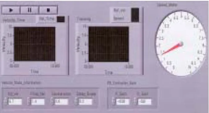
Fig 5. Simulink model for the control system Fig 6. Labview front panel model
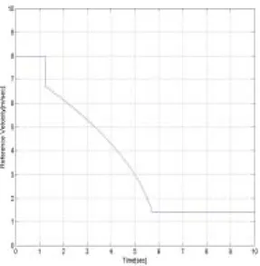
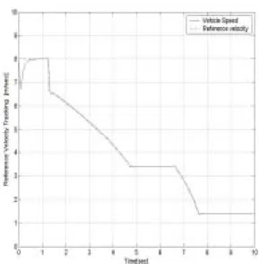
Fig. 5 shows the Simulink model for the simulations. In this figure to calculate the speed profile we need the information of the final speed to be reached, the instantaneous vehicle position by the integration of the vehicle velocity, the block distance or the brick wall safety distance, and the deceleration. It is also necessary to set the vehicle initial velocity for the initial conditions of the simulation. Since we use the equation (10) in this simulation we do not consider the brake activation delay time. However if the traction system has a comparatively long delay time the time to make the brake active should be considered. Fig. 6. is the Labview front panel model communicating with the Simulink model through the TCP/IP port. The vehicle state information block has the parameter values and can be changed in real time while the Simulink model is running. The speed meter displays the transition of the vehicle speed, corresponding to the change of the parameter values. Fig. 7 - Fig. 10 show the simulation results with the different parameter values. Fig. 7 and Fig. 9 are the speed profile produced in the creation of the speed profile block of Fig. 5. We set the final target velocity to 1.4[m/s] in Fig. 7. Fig 8 presents the tracking performance of the proposed control system. As we see in Fig. 8 the vehicle speed follows the reference speed with great performance, which means the AVO module functions very well. In Fig. 9 we set the two different target speeds: one is 3.4[m/s] and the other is 1.4[m/s]. The set of the second target speed is done by the Labview front panel model in real time while the Simulink model is running. With the two different target speed we see two slopes in Fig. 9. First slope is more gradual than the second one because of the large velocity difference from the initial speed to the target speed, which means that the first slope starts from 6.7[m/s] and ends in 3.4[m/s], while the second slope starts from 3.4[m/s] and ends in 1.4[m/s]. Fig. 10 shows the velocity tracking performance for the two target speeds with the significantly good tracking performance. In Fig. 8 and Fig. 10 there are the transient overshoot in the initial states. This is because of the control effort to track the reference velocity which has the non zero initial conditions.
Fig 7. Reference velocity with one target speed
Fig 8. Tracking performance with one target speed
6. Conslusions
In this paper we showed the construction of the control system using Labview Simulation Interface Toolkit and Matlab/Simulink combined system for an application to the personal rapid transit system. The speed profile which has been used in the AVO module as the reference speed was calculated in the speed profile creation block. To guarantee the tracking performance we employed the simple PD compensator. In this paper first, we showed the mathematical model of the traction system using the LDM without considering the resistance for the simplification, and then the equation for the speed profile has been derived. Finally The simulation results showed the effectiveness of the proposed automatic vehicle control system.
REFERENCES
[1]. Jack H. Irving, "Fundamentals of Personal Rapid Transit", Lexington Books, 1978
[2]. Jun-Ho Lee, Ducko Shin, Yong-Kyu Kim, "A Study on the Headway of the Personal Rapid Transit System", Journal of the Korean Society for the Railway, Vol. 8, No. 6, pp. 586-591, 2005.
[3]. Markus Theodor Szillat, "A Low-level PRT Microsimulation", Ph. D. dissertation, University of Bristol, April 2001.
[4]. Duncan Mackinnon, "High Capacity Personal Rapid Transit System Developments", IEEE Transactions on Vehicular Technology, Vol. VT-24, No. 1, pp. 8-14, 1975
[5]. J.E. Anderson, "Control of Personal Rapid Transit", Telektronikk 1, 2003
[6]. Bih-Yuan Ku, Jyh-Shing R. Jang, Shang-Lin Ho, "A modulized Train Performance Simulator for Rapid Transit DC Analysis", Proceedings of the 2000 ASME/IEE Joint Railroad Conference, pp. 213-219, April, 2000.
Fig 9. Reference velocity with two target speed
Fig 10. Tracking performance with two target speed