무선 에너지 전송 센서망에서의 공평성을 고려한 라우팅, 스케줄링, 전력 제어
문 석 재, 노 희 태*, 이 장 원°
Joint Routing, Scheduling, and Power Control for Wireless Sensor Networks with RF Energy Transfer Considering Fairness
Seokjae Moon, Hee-Tae Roh°, Jang-Won Lee*
요 약
최근들어 무선 센서망에서 센서 노드에 대한 전력 공급을 위한 무선 에너지 전송(radio frequency energy transfer: RFET)에 대한 관심이 높아지고 있다. 기존의 센서망에서는 센서 노드들의 에너지 소비를 줄이는 것이 중요한 연구주제 중의 하나였지만 무선 에너지 전송 센서망에서는 센서 노드들이 계속해서 에너지를 공급받을 수 있기 때문에 에너지 소모를 줄이는 것이 상대적으로 그리 중요한 이슈는 아니다. 하지만 센서 노드들 사이에 가용 에너지양의 차가 발생하게 되기 때문에 무선 에너지 전송 센서망의 성능 향상을 위해서는 이와 같은 성질을 고려 하여 프로토콜을 설계하는 것이 중요하게 된다. 이에 본 논문에서는 이를 고려하여 무선 에너지 전송 무선 센서망 에서 라우팅, 스케줄링, 전력제어 기법을 ‘Max-min’과 ‘Max-min fairness’ 두가지의 관점에서 제안을 한다. 또한 본 논문에서 제안한 기법들이 무선 에너지 전송 센서망의 성능을 크게 향상시킴을 보이며 이와 더불어 ‘Max-min’
과 ‘Max-min fairness’ 사이의 차이에 대해서도 논의를 한다.
Key Words : Wireless Sensor Network (WSN), RF energy transfer (RFET), Routing, Scheduling, Power control
ABSTRACT
Recently, radio frequency energy transfer (RFET) attracts more and more interests for powering sensor nodes in the wireless sensor network (WSN). In the conventional WSN, reducing energy consumption of sensor nodes is of primary importance. On the contrary, in the WSN with RFET, reducing energy consumption is not an important issue. However, in the WSN with RFET, the energy harvesting rate of each sensor node depends on its location, which causes the unbalanced available energy among sensor nodes. Hence, to improve the performance of the WSN with RFET, it is important to develop network protocols considering this property. In this paper, we study this issue with jointly considering routing, scheduling, and power control in the WSN with RFET. In addition, we study this issue with considering two different objectives: ‘Max-min’ with which we tries to maximize the performance of a sensor node having the minimum performance and ‘Max-min fairness’ with which we tries to achieve max-min fairness among sensor nodes. We show that our solutions can improve network performance significantly and we also discuss the differences between ‘Max-min’ and ‘Max-min fairness’.
http://dx.doi.org/10.7840/kics.2016.41.2.206
※ 이 논문은 2014년도 정부(미래창조과학부)의 재원으로 한국연구재단의 지원을 받아 수행된 기초연구사업임(2013R1A2A2A0106905 3). The earlier version of this paper, which considered only ‘Max-min’, was presented at ICTC 2014[1].
First Author : Yonsei University Department of Electrical & Electronic Engineering, [email protected], 학생회원
° Corresponding Author : Yonsei University Department of Electrical & Electronic Engineering, [email protected], 종신회원
* LSIS Company Ltd., Anyang, South Korea, [email protected]
논문번호:KICS2015-09-286, Received September 1, 2015; Revised February 10, 2016; Accepted February 22, 2016
Ⅰ. Introduction
It is well known that one of the most important issues in the wireless sensor network (WSN) is the management of energy consumption in each sensor node due to finite and small amount of energy that can be stored in the battery[2]. Hence, most of research efforts in the WSN are devoted to implementing energy efficient network protocols such as medium access control (MAC) and routing protocols assuming that sensor nodes are powered by the battery which cannot be recharged nor replaced easily[3,4].
Recently, with the advance of energy harvesting technologies, energy harvesting from ambient energy sources, such as solar and wind powers, is considered as one of the promising solutions that enable us to operate the WSN without concerning about the depletion of energy in the sensor node[5-7]. However, those ambient energy sources are uncontrollable and unpredictable. Hence, most of research efforts in this area are devoted to dealing with uncontrollable and unpredictable energy harvesting.
More recently, the radio frequency energy transfer (RFET) technology is introduced[8]. In the WSN with RFET, there exists a special node that emits energy with RF signals and sensor nodes are powered by harvested energy from RF signals.
Compared with the ambient energy harvesting technologies, the RFET technology is able to provide reliable, controllable, and predictable energy to each sensor node continuously, and thus, in the WSN with RFET, reducing energy consumption is not an important issue. However, one of the most distinguishing features of the WSN with RFET is that the amount of the harvested energy (energy harvesting rate) of each sensor node strongly depends on its location. More precisely, it strongly depends on the distance between the sensor node and energy emitting node. Due to the unbalanced energy harvesting rates among sensor nodes that depend on the location of each sensor node, maintaining fair energy consumption and fair achieved performance among sensor nodes is more
important to improve the overall system performance in the WSN with RFET. Especially, in many applications in the WSN, their performance depends how often sensed data from each sensor node can be delivered to the sink node, which is strongly related with energy harvesting rates in the WSN with RFET, and we study this issue through joint routing, scheduling, and power control aiming at maximizing the minimum average transmission rate of sensed data among those of sensor nodes in the network.
Especially, routing is a key mechanism to achieve network-wise fairness, since it controls the load (energy consumption) of each sensor node.
Recently, the methods for RFET and network protocols in the WSN with RFET are studied in [9-16]. In [9,10], the methods for RFET from energy transmitters to sensor nodes are studied. In [9], three different techniques for multi-hop energy transfer are proposed. In [10], assuming that there are multiple energy transmitters, the methods for grouping multiple energy transmitters and frequency assignment for each group to transfer RF energy simultaneously are proposed.
In [11-16], network protocols for the WSN with RFET are studied. In [11-13], MAC protocols for the WSN with RFET are studied without considering routing and power control. In [14], the authors design the command sequences between the sink node and sensor nodes. In addition, the command transmission time of the sink node and the charging time of the sensor nodes are obtained based on the charging capability of sensor nodes. In [15], a routing protocol with considering the charging capability of the sensor node is proposed. However, the routing path for each sensor node is selected without considering the routing paths of other sensor nodes, without considering the network-wise performance. Hence, if multiple routing paths choose the same sensor node as their intermediate node, the energy of that sensor node would be exhausted fast.
In [16], the authors propose a routing protocol based on a genetic algorithm in which the base station runs a clustering algorithm and inter-cluster routing algorithm, while sensor nodes update additional cluster adjustment. Contrary to the previous works,
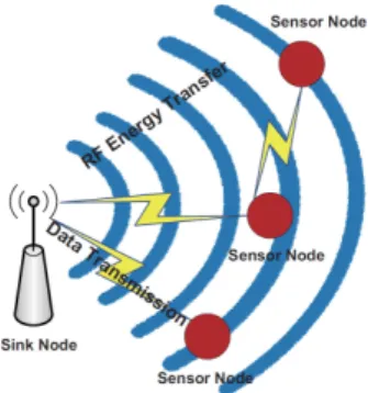
그림 1. RF 에너지 전송 무선 센서망 Fig. 1. Wireless sensor networks with RFET
in this paper, we consider joint routing, scheduling (MAC), power control considering the network-wise performance of the WSN with RFET.
The rest of this paper is organized as follows. In Section II, we introduce the system model for our joint routing, scheduling, and power control for WSNs with RFET. In Section III, we study the problems for ‘Max-min’ and ‘Max-min fairness’.
The numerical results are provided in Section IV and we conclude in Section V.
Ⅱ. System Model
We consider a WSN that consists of one sink node and N sensor nodes as shown in Fig. 1. The sink node will be indexed by 0 and the set of indices for sensor nodes will be denoted by
⋯ . We will denote the set of indices for sensor nodes and the sink by
⋯ . We assume that all nodes are static, i.e., the location of each node is fixed. Sensor nodes transmit their sensed data to the sink node and we allow them to use multi-hop routing via other sensor nodes.
We assume that the system is time-slotted with a fixed duration, , of time-slots, and in a time-slot, a fixed amount of sensed data is transmitted with a fixed data rate. We also assume that a scheduling-based medium access control scheme is used. In addition, since the energy transfer range is relative small compared with communication and interference ranges, we will assume that all sensor
nodes are within the communication and interference ranges of the other nodes. Hence, in a time-slot, only one sensor node is allowed to transmit or forward data. We let be an average scheduling rate of transmissions (the average number of transmissions in a time-slot) from node to node .
Then, we have
∈
∈
≤ ,≥ , ∀∈, ∈. (1)
We define an average net scheduling rate of node
, , as the average number of transmissions of its own sensed data per time-slot. Then, we have the following relationship:
∈
∈
, ∀ ∈. (2)
For the successful transmission, the received signal to noise ratio (SNR) at the receiver node should be higher than or equal to its minimum threshold . In this paper, we assume that the channel gain between two nodes depends only on the path loss. Hence, the received SNR at node from node is obtained as
,
where is a constant that depends on antenna gains of transmitting and receiving antennas, and the wavelength[11], is the transmission power from node to node , is the distance between nodes
and , is the pass loss exponent, and is the noise power. Here, we assume that , , and are fixed and known. To satisfy the minimum received SNR threshold, , the transmission power from node to node should satisfy
≥
. (3)
In addition to the transmission power, we assume
that each node consumes a fixed power, , for receiving data. Hence, the power consumption of each node is formulated as
∈
∈
.
Each sensor node is powered by the RFET from the sink node1) and its transmission power level for energy transfer is assumed to be fixed as . Then, we assume the received power level for energy transfer at sensor node follows the same equation as the received power for data transmissions. Hence,
,
where is some constant that depends on energy harvesting efficiency, antenna gains of transmitting and receiving antennas, and the wavelength[11]. Hence, from the above two equations, for each node
the following condition should be satisfied:
∈
∈
≤, ∀ ∈. (4)
Ⅲ. Problems
In this section, we formulate problems for
‘Max-min’ and ‘Max-min fairness’ considering the system model in the previous section.
3.1 Problem for ‘Max-min’
With ‘Max-min’, the objective of our problem is maximizing the minimum average net scheduling rate among those of sensor nodes in the network, which can be formulated as
∈ . (5)
1) Note that the node that transfers energy need not be the sink node. In addition, our framework in this paper can be easily generalized to the case where multiple RFET nodes exist (possibly at different locations) in the system.
With this objective function and constraints in the previous section, we can formulate the optimization problem that we want to solve in this paper as
∈
∈ ∈
≤
∈
∈ ∀∈
∈
∈≤ ∀∈
≥
∀∈ ∈
≥ ∀∈ ∈
(6)
where ∈, ∈ ∈
, and
∈ ∈
. In the above problem, decision variables are ’s (the average net scheduling rate for node ), ’s (the scheduling rate of transmissions from node to node , which determines routing and scheduling), and ’s (the transmission power from node to node ). Note that
, ∀ ∈ ∈ is an optimal solution of the problem in (6). In the problem in (6), the objective function is nonlinear and non-differentiable. However, we can convert the problem in (6) to the equivalent linear optimization problem by introducing a new variable as
≥ ∀ ∈
∈∈
≤
∈
∈ ∀∈
∈
∈≤ ∀∈
≥ ∀∈ ∈
(7)
We can solve the above linear optimization problem by using one of the standard tools for linear optimization easily. However, the above problem concerns only about the performance of the node that has the minimum average net scheduling rate and does not concerns about the performance of the
Parameter Value Unit
-
-
-
dB
W
W
W
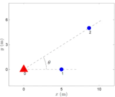
그림 2. 하나의 싱크 노드와 두 개의 센서 노드가 있는 토 폴로지
Fig. 2. A topology with one sink node and two sensor nodes
표 1. 파라미터 설정 Table 1. Parameter setting other nodes. Hence, if we want to care not only the
performance of the node with the minimum performance but also the other nodes’ performance, we need a stronger concept than just maximizing the minimum average net scheduling rate in (5).
3.2 Problem for ‘Max-min fairness’
To consider ‘Max-min fairness’, we first provide the definition of the max-min fairness.
Definition 1[17]: A vector of average net scheduling rates of nodes, ∈ that satisfies (1)-(4) is said to be max-min fair, if for any other vector of average net scheduling rates of nodes,
′ ′ ∈ that satisfies (1)-(4) the following is true: if ′ for some ∈, then there exists
∈ such that ≤ and ′ .
From the definition of the max-min fair, we can easily infer that if is max-min fair, then it achieves (5). In addition, it then maximizes the next minimum one on the condition that it maximizes the minimum one, and so on.
To obtain the max-min fairness, we now introduce a utility function for each sensor node as
, ∀ ∈, (8)
where is a non-negative constant. In [18], it is shown that if we maximize network utility, which is defined as the sum of utilities of all sensor nodes with the above utility function, then the achieved solution approaches the max-min fair solution as
→ ∞ . Hence, considering the above objective function and the system constraints in the previous section, our joint routing, scheduling, and power control problem is formulated as
∈
∈ ∈
≤
∈
∈ ∀∈
∈
∈≤ ∀∈
≥ ∀∈ ∈
(9)
Note that the above problem is a convex
optimization problem, and thus, we can easily solve it by using one of standard algorithms such as dual approach and interior point method[19] or software tools for convex optimization such as the CONOPT solver[20]. Hence, we skip the details.
Ⅳ. Numerical Results
In this section, we provide numerical results to examine the effect of the node position on routing and scheduling with varying the distances between the sink node and sensor nodes. For the sake of easy understanding, we first consider a simple network with one sink node, i.e., node 0, and two sensor nodes, i.e., nodes 1 and 2, as shown in Fig. 2. Node 1 is located at distance 5 (m) from the sink node, i.e., . Node 2 is located at varying distances from 5 (m) to 15 (m) from the sink node, i.e.,
∈ . We set the angle between nodes 1 and 2, i.e., ∠102, to be equal to 30. In addition, we set the parameters which are based on the actual data in [21] as shown in Table I.
Fig. 3 shows the average scheduling rates of each
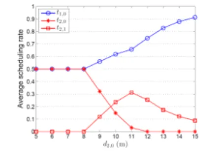
그림 3. 평균 스케쥴링율
Fig. 3. Average scheduling rates 그림 4. 노드 1과 2의 잔여 파워량
Fig. 4. Residual power of nodes 1 and 2 of links with varying distance . When node 2 is
located far from the sink node, i.e., ≥ , it transmits its data to the sink node only via node 1, i.e., and , since its energy harvesting rate is too low to directly transmit its data to the sink node. However, when node 2 is close to the sink node, it can transmit its data directly to the sink node, i.e., , since its energy harvesting rate becomes enough high for direct transmissions.
Fig. 4 shows the residual power of each node ,
, which is defined as the difference between energy harvesting rate (average energy harvesting power) and energy consumption rate (average transmitting power and receiving power):
∈
∈
,
∀ ∈ .
From Fig. 4, we can see that when node 2 is close to the sink node, i.e., ≤ , the residual power of node 2 becomes a positive value. This implies that node 2 harvests enough energy to be fully scheduled. Therefore, as shown in Fig. 3, node 2 transmits its data to the sink node directly without help from node 1, i.e., and and average scheduling rates of nodes are evenly divided. On the other hand, when , node 2 more relies on node 1 for its data transmissions, and thus the average scheduling rate of node 1, , increases, as increases.
We now evaluate the performance of the joint routing, scheduling, and power control with
considering a more general topology in Fig. 5, especially focusing on the effect of routing. In this topology, we have two areas: an inner circle area, which is called a ‘Tier 1’ area, and an outer doughnut area, which is called a ‘Tier 2’ area. We randomly deploy 5 sensor nodes in each of two areas. We set the radius of the Tier 1 area to be 5 (m), and the radii of inner and outer circles of the Tier 2 to be (m) and (m), respectively.
Fig. 6 shows the minimum average net scheduling rates of the network, i.e., ∈ , for different routing policies with varying the value of . The results are obtained by averaging over 100 experiments. In this figure, ‘Max-min’ and
‘Max-min fairness’ represent the minimum average net scheduling rate which are obtained by solving our optimization problems in (7) and (9), respectively. For the problem in (9), we set to be equal to 5 in (8), which is sufficient to achieve almost the max-min fairness 2). Only ‘one-hop’
represents what is obtained with considering only the one-hop transmissions from sensor nodes to the sink node, and ‘Relay from Tier 2 to Tier 1’
represents what is obtained with considering the case where the sensor nodes in the Tier 1 area directly transmit their data to the sink node, while those in
2) In order for the optimal minimum average net scheduling rate of the problem in (9) to be the same as that of the problem in (7), we have to set
to be a very large number (theoretically ∞).
However, when exceeds 5, errors occur due to the permitted limit of the calculable value of the solver that we used (we useed CONOPT solver to solve the convex optimization problem in (7)).
그림 5. 하나의 싱크와 10개의 센서노드가 있는 토폴로지 Fig. 5. A topology with one sink and 10 sensor nodes
그림 6. 각기 다른 여섯 개의 라우팅에서의 최소 평균 순스 케쥴링률
Fig. 6. Minimum average net scheduling rates with six different routing policies
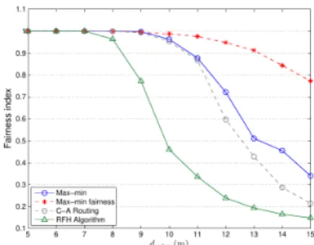
그림 7. 각기 다른 네 개의 라우팅에서의 공평도
Fig. 7. Fairness indices obtained with four different routing policies
the Tier 2 area transmit their data to the sink node only via the sensor nodes in the Tier 1 area., In addition, ‘C-A Routing’ represents what is obtained with the charging-aware routing protocol in which each sensor selects its route with the lowest value of maximum charging time[15] and ‘RFH Algorithm’
represents what is obtained with the routing-first heuristic algorithm in which each sensor node chooses the shortest path to the sink node as its route to minimize the energy consumed by the sensor nodes[22].
From this result, we can see that the solution from the problem in (7) provides almost the same performance as that of the problem in (9) in terms of the minimum average net scheduling rate, even though there exist a small gap between them due to the finite value for that we used in the problem in (7). In addition, the performance of ‘RFH Algorithm’ is identical with ‘Only one-hop’, since each sensor node follows its shortest path which corresponds to direct transmission to the sink node.
The performances of ‘Max-min’ and ‘Max-min fairness’ are always higher than or equal to those of
‘Only one-hop’, ‘Relay from Tier 2 to Tier 1’, and
‘RFH Algorithm’. Note that ‘C-A Routing’ achieves the minimum average net scheduling rate slightly less than that of ‘Max-min’. Hence, if we consider the minimum average net scheduling rate as a sole performance measure of the network, then `C-A Routing’ would be also a good candidate. However, as we will show in the following, its degree of fairness among nodes is worse than those of
‘Max-min’ and ‘Max-min fairness’.
In Fig. 7, we provide the fairness indices of four different routing policies: ‘Max-min’ which is obtained by solving the problem in (7), ‘Max-min fairness’ which is obtained by solving the problem in (7), ‘C-A Routing’, and ‘RFH Algorithm’. We use the following fairness index, which is defined in [23]:
∈
∈
,
where is the number of sensor nodes in the network.
From this figure, we can see that ‘Max-min fairness’ policy always provides a higher fairness index than that of ‘Max-min’, ‘C-A Routing’, and
‘RFH Algorithm’. Therefore, in terms of the fairness between the performances of all sensor nodes,
‘Max-min fairness’ provides a better solution than
the other routing policies. Note that even though
‘C-A Routing’ provides similar minimum average scheduling rate compared to ‘Max-min’, the fairness index of ‘C-A Routing’ is always less than that of
‘Max-min’ and ‘Max-min fairness’. Hence, with both considering minimum average scheduling rate and fairness, ‘Max-min’ and ‘Max-min fairness’
provide better performance than that of ‘C-A Routing’.
Ⅴ. Conclusion
In this paper, we studied the issue of routing, scheduling, and power control exploiting unbalanced energy harvesting rates among sensor nodes in the WSN with RFET. Numerical results showed that in the WSN with RFET, jointly considering routing, scheduling, and power control is essential to improve system performance, while providing fair energy consumption among sensor nodes. In addition, they also showed that ‘Max-min’ and
‘Max-min fairness’ provide almost the same performance from the point of the minimum average net scheduling rate, while ‘Max-min fairness’
provides a higher degree of fairness than ‘Max-min’.
As future work, we can extend our work to a large scale sensor network where a large number of sensor nodes are distributed in a large area. In this case, instead of adopting the centralized scheduling based MAC scheme that we considered in this paper, adopting a distributed random access based MAC scheme, such as CSMA-CA based scheme and slotted ALOHA based scheme, would be a more appropriate approach.
References
[1] H.-T. Roh and J.-W. Lee, “Cross-Layer optimization for wireless sensor networks with RF energy transfer,” ICTC, Oct. 2014
[2] I. F. Akyildiz, W. Su, Y.
Sankarasubramaniam, and E. Cayirci,
“Wireless sensor networks: a survey,” Comput.
Netw., vol. 38, no. 4, pp. 393-422, 2002.
[3] J.-H. Son, S.-G. Shon, and H.-J. Byun,
“Bio-Inspired energy efficient node scheduling algorithm in wireless sensor networks,” J.
KICS, vol. 38, no. 6, pp. 528-534, 2013.
[4] Y.-B. Cho, S.-H. Woo, and S.-H. Lee,
“IDE-LEACH protocol for trust and Eenergy efficient operation of WSN environment,” J.
KICS, vol. 38, no. 10, pp. 801-807, 2013.
[5] A. A. Aziz, D. Tribudi, L. Ginting, P. A.
rosyady, D. Setiawan, and K. W. Choi, “RF energy transfer testbed based on off-the-shelf components for IoT application,” J. KICS, vol.
40, no. 10, pp. 1912-1921, 2015.
[6] W. K. G. Seah, Z. A. Eu, and H.-P. Tan,
“Wireless sensor networks powered by ambient energy harvesting (WSN-HEAP) - survey and challenges,” in Wireless VITAE, pp. 1-5, Aalborg, May 2009.
[7] B. Kim, S. Park, and D. Hong, “Transmission capacity of wireless energy harvesting ad hoc networks,” in Proc. KICS Fall Conf., pp. 256- 257, Seoul, Korea, Nov. 2011.
[8] X. Lu, P. Wang, D. Niyato, D. Kim, and Z.
Han, “Wireless networks with RF energy harvesting: a contemporary survey,” in IEEE Commun. Surveys & Tuts., vol. 17, no. 2, pp.
757-789, 2015.
[9] M. K. Watfa, H. AlHassanieh, and S. Selman,
“Multi-hop wireless energy transfer in WSNs,”
IEEE Commun. Lett., vol. 15, no. 12, pp.
1275-1277, Dec. 2011.
[10] P. Nintanavongsa, M. Y. Naderi, and K. R.
Chowdhury, “Medium access control protocol design for sensors powered by wireless energy transfer,” in IEEE INFOCOM, Apr. 2013.
[11] J. Kim and J.-W. Lee, “Energy adaptive MAC protocol for wireless sensor networks with RF energy transfer,” in ICUFN, Jun. 2011.
[12] J. Kim and J.-W. Lee, “Performance analysis of the energy adaptive MAC protocol for wireless sensor networks with RF energy transfer,” in ICTC, Sept. 2011.
[13] C. Fujii and W. K. G. Seah, “Multi-tier probabilistic polling in wireless sensor networks powered by energy harvesting,” in ISSNIP, Dec. 2011.
[14] J. P. Olds and W. K. G. Seah, “Design of an active radio frequency powered multi-hop wireless sensor network,” in IEEE ICIEA, Jul.
2012.
[15] R. Doost, K. R. Chowdhury, and M. D.
Felice, “Routing and link layer protocol design for sensor networks with wireless energy transfer,” in IEEE GLOBECOM, Dec. 2010.
[16] Y. Wu and W. Liu, “Routing protocol based on genetic algorithm for energy harvesting- wireless sensor networks,” in IET Wireless Sensor Syst., vol. 3, no. 2, pp. 112-118, Jun.
2013.
[17] R. Srikant, The Mathematics of Internet Congestion Control, Birkhauser, 2003.
[18] J. Mo and J. Walrand, “Fair end-to-end window-based congestion control,” IEEE/ACM Trans. Netw., vol. 8, no. 5, pp. 556-567, Oct.
2000.
[19] S. Boyd and L. Vandenberghe, Convex optimization, Cambridge Univ. Press, 2004.
[20] A. Drud, CONOPT solver manual, ARKI Consulting and Development, Bagsvaerd, Denmark, 1996.
[21] Powercast Corporation, TX91501 User’s manual & P2110’s datasheet, Retrieved Nov.
2015, from
http://www.powercastco.com/resources.
[22] B. Tong, Z. Li, G. Wang, and W. Zhang,
“How wireless power charging technology affects sensor network deployment and routing,” in Proc. IEEE ICDCS, pp. 438-447, Jun. 2010.
[23] R. Jain, D. Chiu, and W. Hawe, “A quantitative measure of fairness and discrimination for resource allocation in shared computer systems,” Tech. Rep., Sept. 1984.
문 석 재 (Seokjae Moon)
2012년 8월:연세대학교 전기 전자공학부 학사
2016년 2월:연세대학교 전기 전자공학부 석사
2016년 3월~현재:연세대학교 전 기전자공학부 박사과정(예정)
<관심분야> 통신망 자원 할당, 통신망 최적화
노 희 태 (Hee-Tae Roh)
2005년 2월:연세대학교 전기 전자공학부 학사
2012년 2월:연세대학교 전기 전자공학부 박사
2014년 8월:연세대학교 전기 전자공학부 박사후과정 2014년 9월~현재:LS산전
<관심분야> 통신망 자원 할당, 통신망 최적화
이 장 원 (Jang-Won Lee)
1994년 2월:연세대학교 전기전 자공학과 학사
1996년 2월:한국과학기술원 전 기 및 전자공학과 석사 2004년 8월:Dept. of ECE
Purdue University 박사 2004년 9월~2005년 8월: Dept.
of EE Princeton University 박사 후 연구원 2005년 9월~2010년 8월:연세대학교 전기전자공학부
조교수
2010년 9월~2015년 8월:연세대학교 전기전자공학부 부교수
2015년 9월~현재:연세대학교 전기전자공학부 교수
<관심분야> 통신망 자원 할당, 통신망 최적화, 통신망 성능 분석