2006, Vol. 17, No. 3, pp. 919 925 2006, Vol. 17, No. 3, pp. 919 925 2006, Vol. 17, No. 3, pp. 919 925 2006, Vol. 17, No. 3, pp. 919 925~~~~
MLE for Incomplete Contingency Tables MLE for Incomplete Contingency Tables MLE for Incomplete Contingency Tables MLE for Incomplete Contingency Tables
with Lagrangian Multiplier with Lagrangian Multiplier with Lagrangian Multiplier with Lagrangian Multiplier
Shin-Soo Kang Shin-Soo KangShin-Soo Kang Shin-Soo Kang1)1)1)1)
Abstract Abstract Abstract Abstract
Maximum likelihood estimate(MLE) is obtained from the partial log-likelihood function for the cell probabilities of two way incomplete contingency tables proposed by Chen and Fienberg(1974). The partial log-likelihood function is modified by adding lagrangian multiplier that constraints can be incorporated with. Variances of MLE estimators of population proportions are derived from the matrix of second derivatives of the loglikelihood with respect to cell probabilities.
Simulation results, when data are missing at random, reveal that Complete-case(CC) analysis produces biased estimates of joint probabilities under MAR and less efficient than either MLE or MI. MLE and MI provides consistent results under either the MAR situation. MLE provides more efficient estimates of population proportions than either multiple imputation(MI) based on data augmentation or complete case analysis.
The standard errors of MLE from the proposed method using lagrangian multiplier are valid and have less variation than the standard errors from MI and CC.
Keywords Keywords Keywords
Keywords : Complete case analysis, Multiple imputation, Partial log-likelihood
1. Introduction 1. Introduction1. Introduction 1. Introduction
In the analysis of contingency tables, it may happen that some observations are not fully observed. This issue relating incomplete contingency tables has been studied for a long time. One simple approach, known as complete-case(CC) analysis, discards the missing data by restricting analysis to only fully classified counts in an incomplete contingency table.
1) Professor, Department of Management and Information, Kwandong University, Kangnung, 210-701, Korea
E-mail: [email protected]
Chen and Fienberg (1974) used an iterative procedure for computing maximum likelihood estimates and developed Pearson and likelihood ratio tests of independence for two-way tables for which either the row classification or the column classification could be missing for some cases. As in Chen and Fienberg (1974), Hocking and Oxspring (1974) consider three independent multinomial distributions corresponding to the set of fully cross-classified counts and the two sets of partially classified counts, where either the row classification or the column classification is missing.
An alternative approach involves constructing a complete table, in which all cases are completed classified, by imputing information for the missing row or column classification. Multiple imputation, proposed by Rubin (1978), provides a way to take advantage of commonly used tests of independence for completely classified tables.
West et al.(2002) proposed a method using an EM algorithm and a Bayesian prior to analyze longitudinal studies with repeated measures. They generate all possible sets of missing values, form a set of possible complete data sets, and then weight each data set according to clearly defined assumptions. They apply an appropriate statistical test procedure to each data set, combining the results to give an overall indication of significance.
Instead of imputing information for missing classifications, maximum likelihood estimates of population proportions can be obtained from the observed information, including both the completely and partially classified cases.
Little(1982) used a simple EM algorithm to estimate cell probabilities.
Maximum likelihood estimates of population proportions is obtained from the partial log-likelihood function for the cell probabilities of two way incomplete contingency tables proposed by Chen and Fienberg(1974). This MLE method does work under MAR. Constraints such as sum of cell probabilities is equal to one can be incorporated with lagrangian multiplier proposed by Aitchison and Silvey(1958). Variances of MLE estimators of population proportions are derived from the matrix of second derivatives of the loglikelihood with respect to cell probabilities.
The performances of MLE, MI and the CC approach are examined through the Monte Carlo studies in section 4. The bias and efficiency of estimates of population proportions are considered.
2. Notation and Likelihood Function 2. Notation and Likelihood Function 2. Notation and Likelihood Function 2. Notation and Likelihood Function
Consider an I×J contingency table where the row factor X1 hasI categories and the column factorX2 has J categories. Assume simple random
sampling with replacement. In a complete table, where the row and column categories are observed for every case in the sample, the counts have a multinomial distribution with sample size N and probability vector θ, where θ=(θ11,θ12,⋯θ1J,θ21,⋯,⋯,θIJ). Let θij be an element of θ, denote the population proportion for the cell (i,j).
When information on either the row or column classification is missing, we can construct a table of counts for the completely classified cases wherexij denotes the number of cases observed in the (i,j) cell. We can also construct one-way tables of counts for partially classified cases. Let xim denote the number of cases in the ith row category, i= 1,2,⋯,I, where the column category is unknown, and let xmj denote the number of cases in the jth column category, j= 1, 2,⋯,J, where the row category is unknown. Then, xim and xmj are marginally observed counts on a single variable. Let xmm denote the number of cases where both the row and column categories are missing.
The total sample size is
N = ∑
ijxij+∑
ixim+∑
jxmj+xmm
= xcc+x+m+xm++xmm.
The partial log-likelihood function for the cell probabilities θ proposed by Chen and Fienberg(1974) is the following;
l(θ) =∑
i∑
jxijlogθij+∑
jxmjlogθ+j+∑
iximlogθi+ (1)
The log-likelihood function in (1) dose not include xmm. Discarding the xmm cases for which both variables are missing does not affect any results in this paper except N changed to n=N-x m m because those cases do not contain any information about the joint distribution of X1 and X2.
3. MLE of Cell Probabilities and Its Variance 3. MLE of Cell Probabilities and Its Variance 3. MLE of Cell Probabilities and Its Variance 3. MLE of Cell Probabilities and Its Variance
The EM algorithm can be used to get a MLE. Little(1982) illustrates EM procedure with partially classified data on two variables. The EM algorithm is quite simple. The estimates at tth iteration is
θ(ijt)=1/n
(
xij+xim× θθ((iij+tt- 1)- 1)+xmj× θ(ijt- 1)θ(+t- 1)j
)
, where θ(0)ij =xxccij . The estimates atthe first step of EM procedure. We can get a MLE of θafter convergence.
For the example by Little(1982), the 30 partially classified units with X1= 1 have X2= 1 with probability 100/(100+50) and X2= 2 with probability 50/(100+50). Thus in effect, (30)(100)/150 = 20 are allocated to X2= 1 and (30)(50)/150 =10 are allocated to X2= 2 at the first step. In the next step new cell probabilities are computed from the completed data and the procedure iterates to convergence.
Since we have a constraint such as
∑ijθij= 1, the likelihood function (1) can be expressed with lagrangian multiplier as
l(θ*)=∑
i∑
jxijlogθij+∑
jxmjlogθ+j+∑
iximlogθi++ γ(1-∑
ijθij),
where θ*=(θ',γ)'. The first derivative of l(θ*) with respective to θij and γ is
∂l(θ*)
∂θij = xij θij+ xmj
θ+j+ xim θi+-γ
∂l(θ*)
∂γ = 1-∑
ijθij. The second partial derivatives are
∂2l(θ*)
∂θ2ij = -xij θ2ij - xmj
θ2+j- xim θ2i+ ,
∂2l(θ*)
∂θij∂θis = - xim
θ2i+ , ∂2l(θ*)
∂θij∂θkj =- xmj θ2+j
∂2l(θ*)
∂θij∂θks = 0, ∂2l(θ*)
∂θij∂γ =-1, ∂2l(θ*)
∂γ2 =0
Let I(θ*) be the matrix of second derivatives of the loglikelihood with respect to θ*. An estimate of the covariance matrix of θˆ* which is a MLE of θ* is -I-1( θˆ*). Let ˆΣM be a matrix omitting the last row and column of -I-1( θˆ*). ˆΣM gives us an estimate of the covariance matrix of θˆM, where
θM
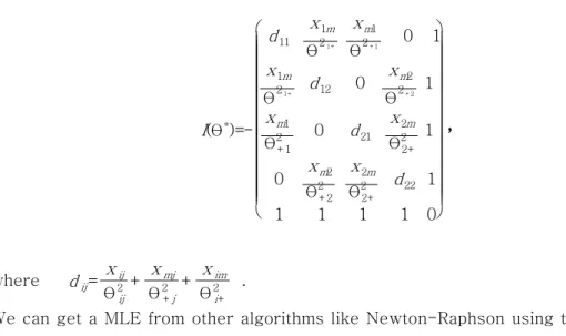
ˆis a MLE of θ computing through EM procedure. For 2 ×2 table, θ*=(θ11,θ12,θ21,θ22,γ)' and I(θ*) is
I(θ*)=-
d11 x1m
θ21+
xm1
θ2+1 0 1 x1m
θ21+ d12 0 xm2 θ2+2 1 xm1
θ2+1 0 d21 x2m θ22+ 1 0 xm2
θ2+2 x2m
θ22+ d22 1
1 1 1 1 0
,,,,
where dij= xij θ2ij + xmj
θ2+j+ xim θ2i+ .
We can get a MLE from other algorithms like Newton-Raphson using the matrix of second derivatives of the loglikelihood with respect to θ* instead of EM algorithm, but both methods provide similar results of MLE.
4. Simulation Results 4. Simulation Results4. Simulation Results 4. Simulation Results
The performances of MLE, MI and the CC approach are examined through the Monte Carlo studies. All of the 2×2 incomplete contingency tables for this study were generated with equal probability margins and sample size N= 500 such that (θ11,θ12,θ21,θ22)=(0.2,0.3,0.3,0.2). There are two cases with different missing at random mechanism(MAR) and 1000 tables were generated for each case. The missing mechanism for each case is
Pr(X1ismissing |X2=1) = m1 Pr(X1ismissing |X2=0) = m2 Pr(X2ismissing ) = m3
(2)
For the first case m1= 0.1, m2= 0.3, m3= 0.2 and for the second case m1=0.2, m2= 0.4, m3= 0.3 in (2), respectively. The percentages of cases with missing information on at least one variable are expected to be 36%
and 51% for case 1 and 2 respectively. We will compare three methods to check point estimations of θ11 and θ1+θ+1-θ11 and standard errors of θˆ11.
The algorithms for MI were programmed through S-PLUS 6.1(2001) functions for missing values.
Table 1 shows means and standard deviations of 1000 values for the estimates of θ11 from the generated 1000 tables in this section. The true value of θ11 is
0.2. MLE and MI methods provide essentially unbiased estimates for the cell probabilities but CC does not. The standard deviations of the estimates differ across methods. Complete-case analysis provides the estimate of θ11 with the largest variance. For all methods, variation increases as the proportion of missing values increases. MLE tends to provide smaller standard deviations of cell proportion than MI.
MLE MI CC
Case Mean S.D. Mean S.D. Mean S.D.
1 0.1984 0.02063 0.1988 0.02118 0.2242 0.02377 2 0.1978 0.02193 0.1977 0.02281 0.2281 0.02697
<Table 1> Point estimation of θ11
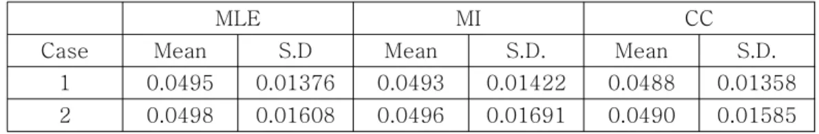
Table 2 shows means and standard deviations of 1000 simulated values for the estimates of θ1+θ+1-θ11, a measure of association between the two variables, when the true value of θ1+θ+1-θ11 is 0.05. The averages of the estimates are similar for all methods. The complete-case and MLE have similar standard deviations and they exhibit smaller standard deviations than MI.
MLE MI CC
Case Mean S.D Mean S.D. Mean S.D.
1 0.0495 0.01376 0.0493 0.01422 0.0488 0.01358 2 0.0498 0.01608 0.0496 0.01691 0.0490 0.01585
<Table 2> Point estimation of θ1+θ+1-θ11
Table 3 shows means and standard deviations of 1000 standard errors of ˆθ11. The averages of the standard errors are close to standard deviations of θ11 in Table 1 for all methods. It says that all three methods provides valid standard errors. The standard errors of MLE obtained from the matrix of second derivatives of the loglikelihood have less variation than the standard errors from MI and CC. MI standard errors have the largest variation among three methods.
MLE MI CC
Case Mean S.D Mean S.D. Mean S.D.
1 0.0202 0.00080 0.0206 0.00188 0.0233 0.00099 2 0.0222 0.00094 0.0227 0.00322 0.0268 0.00128
<Table 3> Standard errors of θˆ11
5. Conclusion 5. Conclusion 5. Conclusion 5. Conclusion
It has been an issue to estimate the variance of MLE for the cell probabilities of an incomplete contingency table because it is very complicated to get the second derivatives of the likelihood. The likelihood with lagrangian multiplier can solve this problem. The standard errors of MLE obtained from the matrix of second derivatives of the loglikelihood are valid and have less variation than the standard errors from MI and CC.
Complete-case(CC) analysis produces biased estimates of joint probabilities under MAR and less efficient than either MLE or MI. MLE and MI provides consistent results under either the MAR situation.
When data are missing at random, simulation results reveal that MLE provides more efficient estimates of population proportions than either multiple imputation(MI) based on data augmentation or complete case analysis, but neither MLE nor MI provides an improvement over complete-case(CC) analysis with respect to θ1+θ+1-θ11, which is a measure of association between the two variables.
References References References References
1. Aitchison, J., and Silvey, S. D. (1958). Maximum-Likelihood Estimation of Parameters Subject to Restraints,The annals of Mathmatical
Statistics, 29, 813-828.
2. Chen, T. T., and Fienberg, S. E. (1974). Two-dimensional contingency tables with both completely and partially cross-classified data,
Biometrics, 32, 133-144.
3. Hocking, R. R., and Oxspring, H. H. (1974). The Analysis of Partially Categorized contingency Data, Biometrics, 30, 469-483.
4. Little, R. J. A., and Rubin, D. B. (2002). Statistical analysis with missing data, J. Wiley and Sons, New York.
5. Rubin, D. B. (1978). Multiple Imputation in Sample Surveys - A Phenomenological Bayesian Approach to Nonresponse, Proceedings of the Survey Research Methods Section, American Statistical Association, 1978, 20-34.
6. S-Plus 6.1 Manual: Analyzing Data with Missing Values in S-Plus (2001). Insightful Corporation. Seattle, Washington.
7. West, C. P., and Dawson, J. D. (2002). Complete imputation of missing repeated categorical data: one-sample applications, Statistics in Medicine, 21, 203-217.
[ received date : Jun. 2006, accepted date : Jul. 2006 ]