Nonparametric Test for Money and Income Causality

2004, Vol. 15, No. 2, pp. 485∼493

Nonparametric Test for Money and Income Causality¹⁾

Kiho Jeong²⁾

Abstract

This paper considers the test of money and income causality. Jeong (1991, 2003) developed a nonparametric causality test based on the kernel estimation method. We apply the nonparametric test to USA data of money and income. We also compare the test results with ones of the conventional parametric test.

Keywords : cointegration, Granger-causality, kernel, nonparametric test, unit root,

1. Introduction

Whether movements in money help predict movements in income is an important question to the formulation of monetary policy. Accordingly, the response pattern of income to money has been the object of much research attention in empirical macroeconomics.³⁾

Since Sims' (1972, 1980) works, empirical investigations into this relation have been done in the context of "Granger Causality" in either a bivariate or multivariate framework.⁴⁾ In bivariate framework, the approach employed in virtually all of these studies is to assume a linear model, to regress the current income on past incomes and past money supplies, and to test the null hypothesis that the coefficients on past money supplies are all zero. However, this approach is highly likely to miss any nonlinear relationships between money and income.

Jeong(1991, 2003) proposed a nonparametric causality test which does not require

1) This research was supported by Kyungpook National University Research Fund, 2000 The author would like to thank two referees for helpful comments.

2) Professor, School of Economics and Trade, Kyungpook National University, Taegu 702-701, Korea

E-mail: [email protected].

3) For a survey of recent literature, see Stock and Watson (1989).

4) For various concepts of Granger causality, see Granger(1988).

parametric specification of the regression functions. The test uses nonparametric kernel method to estimate the time series regression functions. Jeong(1991, 2003) derived asymptotic normal distribution for the test statistic under the condition of strong-mixing.

In this paper, we apply Jeong's nonparametric causality test to USA data of money and income. For purpose of comparison, we perform the conventional parametric causality test. The obtained result will be compared with the result of nonparametric causality test.

In the next section, we provide parametric test results. In section 3, we briefly describe Jeong's nonparametric causality test and provide the nonparametric test results. Section 4 contains conclusion.

2. Parametric Causality Test

In this section, we perform the conventional parametric causality test. The obtained result will be compared with the result of nonparametric causality test given later. In the context of a bivariate framework, the Granger-causality in mean is defined as follows:

(i) M does not cause Y in mean with respect to U_{t - 1} if

E (yt| U_{t - 1}) = E ( y_t| U_{t - 1}- M_{t - 1}) and (1) (ii) M is a prima facie cause in mean of Y with respect to Ut - 1 if

E (y_t| U_{t - 1}) ≠ E ( y_t| U_{t - 1}- M_{t - 1}), (2)

where M and Y are time series of money and income, M_t is M 's entire histories up to and including time t with M_t= { m_{t - s}, s≥0} and U_t is an information set available at time t.

The conventional approach to testing Granger-causality is to replace the conditional expectations in the definition of causality with linear least-square projections. We take the work of Stock and Watson (1989) as a representative example on this line and replicate their results with extended sample (the sample period used in Stock and Watson (1989) being 1959.1 - 1985.12).

The data consist of monthly observations on the log of seasonally adjusted nominal M1 (m) and the log of seasonally adjusted industrial production total index (y), obtained from the Citibase's data base. The name of each series in the data base is FM1 and IP, respectively. Units are billions of dollars for the M1 and the year of 1977 = 100 for the industrial production index. Sample period covers from January 1959 to September 1989, resulting in a sample size of 369.

Since the asymptotic distributions of the conventional parametric causality tests

are sensitive to unit roots and time trends in the series (Sims, Stock and Watson ,1990), we first characterize the time trend and unit root properties of the data.

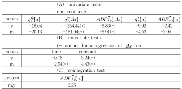
Table 1 displays the results. The first column shows the results of testing a single unit root when there might be a quadratic time trend; i.e., for x = y, m, the hypotheses to be tested are

<Table 1> Tests for integration, cointegration and time trends (A) univariate tests

unit root tests

series q^τ2_f [x] q^τ_f[Δx] ADF τˆ[ Δx ] _τ q^τ_f[ x] ADF τˆ[ x ] _τ y -16.04 -154.44(*) -5.83(*) -9.92 -2.42 m -20.13 -181.94(*) -5.91(*) -4.53 -2.95

(B) univariate tests

t-statistics for a regression of Δ x on series time constant

y -0.78 3.24(*) m -2.54(*) 4.43(*)

(C) cointegration test

system ADF τˆ[ x ]_τ

m,y -2.25

※ Note: All statistics are based on regressions with six lags. q^τ2_f [x] denotes the Stock and Watson (1989) q^τ2_f (1,0)-statistic computed using the level of each variable; q^τ_f[ Δx]

denotes the Stock and Watson (1988) q^τ_f(1,0)-statistic computed using the first difference of each variable; ADF τˆ[ Δx ]_τ denotes the Dickey-Fuller t-statistic computed using the first q^τ_f[x] ^and ˆ[ x ]τ_τ . Critical values for the ˆτ_τ-statistic are from Fuller (1976, p.373); for the q^τ2_f (1,0)-statistic from Stock and Watson (1989). (*) denotes being significant at the 1%

level.

H₀: φ( L)( 1 - L)( x_t-a₀-a₁t-a₂t²)= εt (3) H₁: φ( L)( 1 - ρL)( x_t-a₀-a₁t-a₂t²)= ε_t , ∣ρ∣ < 1

where L is the backshift operator, εt is a series of zero mean, finite variance iid random shocks, and φ(L)= 1-φ ₁L-..-φ_pL^p. The employed test is the Stock-Watson(1989) q_f^{τ 2}-test. In no case is there significant evidence against the unit root hypothesis. The next two columns present the results of Stock-Watson (

1988)'s q^τ_f-test and Augmented Dickey-Fuller test for a second unit root, i.e., for a unit root in the first difference of the series, allowing for the alternative that the series is stationary in first differences around a linear time trend: For x = y, m,

H₀: φ( L)( 1 - L)( Δx_t-a₀-a₁t ) = ε_t (4) H₁: φ( L)( 1 - ρL)(Δx_t-a₀-a₁t ) = ε_t , ∣ρ∣ < 1

These tests suggest that no series contains two unit roots.

The distribution of the test statistics under the null hypothesis depends on the specification of the deterministic part. To ascertain the order of the deterministic components in the specification, the first difference of each series was regressed against a constant, time and six of its own lags (the latter to obtain correct standard errors); For x = y, m,

Δx_t= a₀+ a₁t+ a₂Δ x_{t - 1}+ …+ a₇Δ x_{t - 6}+ε_t (5) The t-statistics on the time trend are reported in the first column of panel B of Table 1. Money growth ( Δm) turns out to have a significant deterministic trend.

Performing the same test without a time trend (column 2) indicates that output has a significant drift.

Since output growth ( Δy) does not appear to exhibit deterministic time trend, the fourth and the fifth columns of panel A of Table 1 report tests for a single unit root, allowing for the alternative that the process is stationary around a linear time trend : For x = y, m,

H₀: Φ( L)( 1 -L) ( x_t- a₀- a₁t ) = ε_t (6) H₁: Φ( L)( 1 - ρL)( x_t- a₀- a₁t ) = ε_t, | ρ | < 1.

Again, all tests give the expected results: The null of a unit root is not rejected. It is concluded that, over the 1959. 1 ∼ 1989. 9 sample, y is well described as process having a single unit root with drift; m has a single unit root with quadratic time trend.

It is well known that a bivariate co-integrated system must have a causal ordering in at least one direction and, without the cointegration being explicitly considered, the model will be misspecified (Engle and Granger, 1987; Granger, 1988). Panel C of Table 1 reports the result of test for the cointegration between money and income.

The test procedure followed Engle and Granger(1987), with the Augmented Dikey-Fuller test used. However, the test fails to reject the null of non-cointegration.

In sum, the foregoing discussion suggests the following specification:

Δy_t= a₀+ Δη_t (7) Δm_t= b₀+ b₁t+ Δμ_t

where Δ η_t and Δ μ_t are mean zero stationary processes.

To perform the conventional parametric test for Granger-causality, consider the following Δ y_t equation in a bivariate VAR(p) of Δ μ_t and Δ y_t :

Δy_t= α₀+ α_m(L) Δμ_t+ α_y(L) Δy_t+ ε_t . (8) The null hypothesis to be tested is that the deviation of money growth from a linear time trend ( Δμ) does not Granger-cause growth in the industrial production index( Δy); i.e., αm(L) = 0 in equation (8). Since Δ y_t and Δ μt do not contain unit roots, the usual procedure of F-test is valid and is reported in Table 2. As in Stock and Watson(1989), all regressions were based on regression with 6 lags of each variables. Interestingly, the test does not reject the null of non-causality.

This result does contradict with Stock and Watson's(1989) finding that robust to changes in the sample period, the derivation of money growth from a linear time trend Granger-causes growth in the industrial production index. This suggests that it may be worth replicating their other results with the extended sample size.

However, it is not a major concern in this study, thus we do not pursue the topic further.

<Table 2> Parametric causality test

specification SSE F(6,349)-statistic Δy_t= α₀+α_y(L)Δy_t+ ε_t

Δy_t= α₀+α_m(L)Δm_t+α_y(L)Δy_t+ ε_t

0.0258

0.0251 1.6222

※ All regressions are based on regression with 6 lags of each variable. SSE denotes sum of squared errors.

3. Nonparametric Causality Test

We now perform Jeong(1991, 2003)'s nonparametric causality test. We note that if we assume U_{t - 1}= Y_{t - 1}∪^Mt - 1= { y_{t - 1},.., y_{t - p}, m_{t - 1}, .. , m_{t - q}} then, from the definitions (1) and (2), the hypotheses of causality test are specified as

H_o: E ( y_t| y_{t - 1},., y_{t - p}, m_{t - 1},. , m_{t - q}) = E ( y_t| y_{t - 1},.., y_{t - k}) (9) H₁: E ( y_t| y_{t - 1},.., y_{t - p}, m_{t - 1}, .. , m_{t - q}) /= E ( y_t| y_{t - 1},.., y_{t - k}). (10)

Thus, L2- measure comparison of nonparametric estimators of two conditional expectations in equation (9) can be one way to test (9) against (10). For notational simplicity, we define

z_t≡ ( y_{t - 1},.., y_{t - p}, m_{t - 1}, .. , m_{t - q}), (11)

x_t≡ ( y_{t - 1},.., y_{t - p}) (12)

k ≡ p + q . (13)

v_Tt ≡ { y _{t + T / 2}- E ( y_{t + T / 2}| zt + T / 2 - 1) }²1 { f ( zt + T / 2 - 1) > b_T} - { y_t- E ( y _t| z_t) }²1 { f ( z_t) > b_T} and (14) σ²≡ lim

T→∞Var

{

}

Jeong(1991, 2003)'s nonparametric test is based on the following statistic;

Mc˜ _{= T}^{- 1}_{∑wt⋅(yt- Eˆ (yt| xt))}²_{⋅1(fˆ ( zt) > bT)}

- T^{- 1}∑^{( 1 - w}t)⋅(^{yt- Eˆ (yt| zt)})^2⋅1(^{fˆ ( zt) > bT}), (14)

where Eˆ (y_t| ⋅ ) denotes the common Nadaraya-Watson kernel estimator defined as

ˆ (yE _t| z_t) =

T^{- 1} ∑

T

s = 1h^{- k}_T K

(

)

T^{- 1}∑

T

s = 1h^{- k}_T K

(

)

value of fˆ (z ) than bT are trimmed out to prevent erratic behavior of M˜_c. Jeong(1991, 2003) showed the following asymptotic results hold for the statistic M_c

˜;

( 2 T )^{1 / 2}σ^{- 1}˜M

c → N ( 0 , 1 ) in distribution and (16)

s²_Tl → σ² in probabiltity (17)

where s²_Tl ≡ ( T / 2 )^{- 1} ∑^{T / 2}

t = 1ˆv²

Tt+ 2 ∑^l

s = 1ω

(

)

Ttˆv

Tt - s, ˆv

Tt≡ {^{yt + T / 2- Eˆ (y t + T / 2| z}t + T / 2 - 1)}^2⋅1{^{fˆ ( z}t + T / 2 - 1) > b_T}

-{^{yt- Eˆ (yt| zt - 1)}}^2⋅1{^{fˆ ( z t - 1) > bT}}^,

ω ( ⋅ ) is a real-valued kernel and l ≤ T / 2 is a lag truncation parameter; the sample autocovariance functions ( T / 2 )^{- 1} ∑^{T / 2}

t = s + 1ˆv

Ttˆv

Tt - s receive weight ω ( ⋅) for lags of order s ≤ l , but zero weight for s > l . The motivation for this estimator is that for a stationary random sequence the long-run variance σ² equals 2 π times the spectral density evaluated at zero and the estimators s²Tl is the value at frequency zero of 2 π times an estimator for the spectral density of v_Tt, where the kernel weights are used to smooth the sample autocovariance functions (Hansen, 1982; Newey and West, 1987).

In practice, one should choose the lag structure of the information set Ut, kernel functions K₀ and K₁, bandwidth parameters h_0T and h_1T, trimming bound bT, sample splitting scheme wt and the lag order l. To compare with result from the conventional test, we assume that the information set U_t contains the 6 lagged variables of each Δμ and Δy:

U_t = { Δyt - 1, …, Δyt - 6, Δmt, …, Δmt - 5}, (18) thus implying that z_t = ( Δyt - 1,……, Δyt - 6, Δmt, ……, Δm_{t - 5}) and

x_t = ( Δy_{t - 1},……, Δy_{t - 6}).

Among standard positive kernel functions, I chose the standard normal density function for both K₀ and K₁:

K( u) = 1

2π exp

(

)

For the bandwidth parameters, h_0T= 0.0044 and h_1T= 0.0039 are chosen for estimating E( y∣x) and E( y∣z) respectively. These choices are the cross-validation estimates of the bandwidth parameters for estimating the conditional means. In this study, two observations at each boundary of the density estimate fˆ (z) are trimmed, implying about 1% trimming.

As a sample splitting scheme, the first half observations are used to compute the alternative part of the test statistic and the last half are used for the null part. The several values are considered for lag order l; 1, 13, 15 and 24. These numbers are selected on the basis of ACF of ˆv

Tt.

The results of computing test statistic (2 T )^{1 / 2}s_Tl^{- 1}˜M

c are given in Table 3.

Like the result of the parametric causality test, the nonparametric test does not reject the null of non-causality. Thus, we tentatively accept the conclusion that over the sample period 1959.1-1989.9, the deviation of money growth from a linear time trend does not Granger-cause growth in the industrial production, either linearly or nonlinearly.

<Table 3> Nonparametric causality test test

statistic

lag orders ( l )

1 13 15 24 (2 T )^{1 / 2}s_Tl^{- 1}˜M

c 1.21 1.18 1.18 1.19

4. Conclusion

In this paper, we applied Jeong(1991,2003)'s nonparametric causality test to USA data of money and income. For purpose of comparison, we performed the conventional parametric causality test. The null hypothesis that the deviation of money growth from a linear time trend does not Granger-cause growth in industrial production was not rejected. The same result was obtained from conventional parametric causality test which was performed for the purpose of comparison. However, before reasonable conclusions can be reached, further analysis must be done regarding practical implementation of the nonparametric test. Thus, if any, contribution of this paper would be to suggest an example of application for the nonparametric test, in which the process to compute of the nonparametric test statistic is shown.

In particular, small sample properties of the proposed tests were not investigated via simulation study. Thus, the performance of the tests in small samples is not yet known. In addition, the issues of how to choose the lag structure of the

information set Ut, the bandwidth and trimming parameters, and sample-splitting scheme in practice need be studied further. We leave these kinds of issues to further research.

References

1. Engle, R.F. and C.W.J Granger (1987), Cointegration and error correction:representation, estimation and testing, Econometrica, 55, 251-276.

2. Granger, C.W.J (1988), Some recent development in a concept of causality, Journal of Econometrics, 39, 199-211.

3. Hardle, W. (1990), Applied nonparametric regression, Cambridge:

Cambridge University.

4. Hansen, L.P. (1982), Large sample properties of generalized method of moments estimators, Econometrica, 50, 1029-1054.

5. Jeong, K. (1991), Model misspecification tests of regression functions, unpublished Ph.D. Thesis, University of Wisconsin at Madison

6. Jeong, K. (1996), Kernel estimators of 2 pi times the spectral density at frequency zero of nonparametric regression errors, Journal of Economic Theory and Econometrics, 2, 125-135

7. Jeong, K. (1997), Prewhitened kernel estimators of 2 pi times the spectral density at frequency zero of nonparametric regression errors, Journal of Economic Theory and Econometrics, 3, 107-122.

8. Jeong, K. (2003), Nonparametric Granger causality test, presented at 2003 Conference of Korean Economic Association.

9. Newey, W.K. and K. West (1987), A simple, positive semidefinite, heteroscedasticity and autocorrelation consistent covariance matrix, Econometrica, 55, 703-708.

10. Sims, C.A. (1972), Money, income and causality, American Economic Review, 62, 540-552.

11. Sims, C.A. (1980), Macroeconomics and reality, Econometrica, 48, 1-48.

12. Sims, C.A., J.H. Stock and M.W. Watson (1990), Inference in linear time series models with some unit roots, Econometrica, 58, 113-144.

13. Stock, J.H. and M.W. Watson (1988), Testing for common trends, Journal of the American Statistical Association, 83, 1097-1107.

14. Stock, J.H. and M.W. Watson (1989), Interpreting the evidence on money- income causality, Journal of Econometrics, 40, 161-181.

[ received date : Dec. 2003 , accepted date : May. 2004 ]