Geographic Difference in the Prevalence of Osteoporosis in Korea

(1)

Geographic Difference in the Prevalence of Osteoporosis in Korea

Nam Han Cho, Chul Shin

¹

, Chan Park

²

, Kyu Chan Kimm

²

Department of Preventive Medicine, Ajou University School of Medicine, Suwon, Korea Department of Internal Medicine, Korea University College of Medicine, Ansan, Korea

¹

Korean National Genome Institute, Seoul, Korea

²

목적: 지역사회 일반 인구 대상에서의 요골과 경골 골다공증 유병률 분석

방법: 본 연구는 전향성연구로 경기도 소재의 안성과 안산 지역에서 40～69세 남녀 총 10,038명 (남=4,762명, 여

=5,276명)을 대상으로 농촌-도시 지역의 골다공증 유병률을 분석하여 비교하였다. 골다공증 진단은 세계보건기구의 진단 기준에 따랐으며 경골과 요골에서의 골다공증 유병률을 분석 평가하였다. 골다공증 측정은 초음파방법을 사용 하였다.

결과: 농촌 지역인 안성 거주자들의 평균 연령은 55.5±8.8년, 도시 지역인 안산은 49.1±7.9년으로 농촌지역의 평균 연령이 높았다. 성별 분포는 도시의 경우 남녀가 50.3%, 49.7%으로 유사한 분포이며 안성은 여성이 55.4%였다. 체 질량지수는 농촌이 도시 지역에 비해 의미있게 높았다 (안성-24.7±3 kg/m

²

, 안산-24.4±3.3 kg/m

²

, P＜0.01). 거주 기간은 41년 (안성)과 13년 (안산)으로 농촌에서의 거주 기간이 많았다. 혈압과 중성지방을 제외한 모든 검사 수치는 도시 지역에서 높게 분석되었다. 초음파를 사용한 평균 요골 SoS는 농촌 지역에서 높은 수치를 보인 반면 경골은 도시지역에서 높게 나타나는 현상을 보였다. 평균 초경 나이 역시 도시 지역에 비해 농촌 지역 여성에서 늦게 시작 되는 것으로 분석되었다 (16.1±0.9년, 15.6±2년, P＜0.001). 하루 평균 칼슘 섭취량, 음주량, 커피, 탄산음료, 녹차 섭취량은 도시지역 여성들에서 높은 반면 농촌군에서는 흡연량이 높고 운동량은 적은 현상을 보였다. 남성에서는 지역적 차이가 없었다. 두지역간의 골다공증 유병률은 연령-성별-인구분포를 표준화된 방법으로 비교 분석하였다.

경골 골다공증의 경우 도시지역에서 11.4% (남=1.7%, 여=20.8%), 농촌 지역은 8.8% (남=2.2%, 여=15.1%)의 분포를 보여 도시 지역에서 유병률이 높게 나타났으나, 요골 골다공증은 도시지역 7.5% (남=3%, 여=11.9%), 농촌 지역 7.3% (남=3.3%, 여=11.1%)로 유사한 분포를 보였다. 다중로지스틱 회귀분석을 통해 성별, 나이, 체질량지수, 혈압을 보정할 경우 요골골다공증은 농촌지역이 도시지역에 비해 3.3배 (95% 신뢰구간 2.4～4.7, P＜0.0001) 높은 것으로 분석되었다. 이러한 관계성은 경골에서도 농촌군에서 3.7배 (95% 신뢰구간 2.5～5.5, P＜0.0001) 높은 것으로 분석 되었다.

결론: 요골, 경골 골다공증의 중요한 병인요소는 나이, 성별, 혈압, 체질량지수와 농촌 거주로 규명되었다. 특히 고위 험군으로 나타난 50대 이후 농촌 거주 여성들에서의 조속한 중재가 요구되고 있어 골다공증 조기 진단 및 관리가 체계적으로 이루어져야 할 것이다.

중심단어: 농촌-도시, 유병률, 골다공증, 대한민국, 전향성연구

책임저자 : 조남한, 아주대학교 의과대학 예방의학교실

Tel: 031)219-5900, Fax: 031)219-5901, E-mail: [email protected]

(2)

Rural and urban dwelling differ in the incidence of chronic disease such as coronary heart disease and some cancers

^1～3

. These differences might be direct and indirectly related to various environmental factors that one individual is exposed to long period of time.

However, it is very difficult for one to identify the specificrisk factors that are responsible for specific disease. Furthermore, most of chronic diseases are caused by the multiple risk factors. Therefore, in some disease, it is better to evaluated the risk factors as a whole e.g., environment, than try to identify the individual risk factors. Osteoporosis is the one of the key example disease in this matter because it is related to lifetime exposure to the risk factors. Osteo- porosis is a silence, systemic chronic disease that can affect different bones but usually not detected until the fracture of bone

⁴

. Osteoporosis is the leading cause of serious morbidity and functional loss in the elderly population, and it results in 1.5 million fractures and over $10 billion in medical expenditures annually

^5～8

. Osteoporosis affects 28 million Ameri- cans and The National Osteoporosis Foundation estimates 1.5 times increases by year 2015. Medical communities are estimating that osteoporosis is likely to become the most common disorder of our aging population. Thus, understanding of factors that affect the incidence of osteoporosis is critical if we are to successfully minimize the impact of this disorder on morbidity, mortality, and the cost of health care.

Osteoporosis can result patho-genetically from inadequate peak bone mass, excessive bone resorption, or impaired bone formation. These can be affected by genetics, nutrition, lifestyle, systemic hormones, and local factors as well as residential factors. The relative importance of these mechanisms is not fully under- stood and may differ among subjects

⁹

. However, osteoporosis is more common in women than men, especially postmenopausal women. In Kwang-ju city, Korea, the prevalence of osteoporosis and osteopenia according to decades showed a clear difference bet-

ween genders, the prevalence of osteoporosis over 50 years of age being about 3 times higher in women than men. In addition to gender, numerous epide- miologic studies reported that age is one of the most significant and independent risk factor for osteopo- rosis

^10～12

. However, there are still more risk factors are yet to be identified and understand its role for osteoporosis. For example, several studies reported geographic differences in the prevalence of osteo- porosis. The study from Japan indicated that serum vitamin K2 level difference are the reasons for the geographic differences within country

¹³

, however, the European multinational study indicated that anthropo- metric variability are the reasons for geographic differences in the osteoporotic fracture

¹⁴

.

Over 40% of adult peak bone mass is acquired during adolescence. During this period, in order to prevent bone loss the lifestyle choices including ensuring adequate dietary Ca, regular weight-bearing exercise and avoiding hormonal insufficiency, are especially important

¹⁵

. Therefore, both adequate nutri- tion and exercise are essential for development of peak adult bone mass and maintenance of bone during aging. The optimal dietary level of a nutrient may vary from individual to individual and may change with age, intake of other nutrients, disease, drug therapy, or sex hormone status

¹⁶

. Therefore, for better understanding of osteoporosis it is important to eva- luate whether these factors are present independent of geographic variations.

It is very clear that the prevalence of osteoporosis in Korea steadily increased with an economic develop- ment of the nation. Therefore, in order to implement an effective prevention or intervention strategy for osteoporosis, understand the lifetime bone health such as changing pattern and magnitude is very essential.

However, it is very difficult to assess the life time

bone health pattern because of difficulty of measure-

ment, cost, especially in normal community popu-

lation. Thus, in this study we under took the issue by

(3)

using a non-invasive bone quality measuring instru- ment at the multiple bone sites and we investigated au urbanization as the risk factor for osteoporosis and conducted comparative study between the urban and rural area in a large scale community based epide- miologic study in Korea.

Methods 1. Study population

Two communities in South Korea were selected;

the Ansungcohort represented a rural community, and the Ansan cohort an urban community. Both commu- nities were selected for the Korean Health and Genome Study (KHGS) in 2001. Ansung is a far- mland with 90% of participants is involved rice farming, pear or grape orchard, and dairy farming.

Ansan is a mid-size industrial city with 60% of them working as either blue or white collar type of works.

This is an ongoing prospective study involving a biennial examination. Details of the KHGS and the method used have been previously described

¹⁷

. In brief, a total of 10,038 subjects aged from 40 to 69 years were recruited (5,018 from a farming commu- nity, Ansung and 5,020 from an industrial community, Ansan). Of these 10,038 subjects, 5,018 Ansung sub- jects were recruited from a 5 out 11 Myon (lowest governing district) by cluster sampling method. For Ansan, a total of 5,020 subjects were recruited via Systematic Random Sampling method using the telephone directory. A total recruitment rate was about 80%. The study protocol was approved by the Ethics Committee of the Korean Heath and Genomic Study of the Korean National Institute of Health.

2. Measurement of anthropometric and bio- chemical parameters

Height, body weight, waist and hip circumference

were measured standard method in light clothes. Body mass index (BMI) was calculated as weight divided by height squared (kg/m

²

). Body fat and lean body mass were measured by tetrapolar bioelectrical impedance analysis (Inbody 3.0

^Ⓡ

, Biospace, Korea).

Bioelectrical impedance analysis measures two para- meters, fat and lean tissue, using empirically derived formulas that have been validated by earlier studies, and which were found to correlate well with under- water weighing, except for extremely obese sub- jects

^18,19

.

The morning blood pressure was recorded three times between 7 and 9 am, after subjects had been in a relaxed state for at least 10 minutes, 5 minutes resting period was given between the each measure- ment. After 8～14 hours overnight fasting, plasma concentrations of glucose, insulin, total cholesterol, triglyceride, and HDL-cholesterol were measured enzymatically using a Hitachi 747 chemistry analyzer (Hitachi, Tokyo, Japan). The level of LDL-cholesterol (mmol/l) was calculated by using the following formula: [total cholesterol (mmol/l) - HDL-cholesterol (mmol/l) - triglyceride (mmol/l)/2.2)]

²⁰

.

Smoking status was divided into never smoker, ex-smoker, and current smoker (ie., ＜1 pack/day and

≥ 1 pack/day). The term “never” means the person who never smoked in his or her life time and “ever”

was used to classify the person who had smoked for at least one month or currently smokes. Responses to frequency questionnaire were obtained alcohol con- sumption, coffee intake, carbonated beverages consump- tion, dairy products intake and physical exercise.

Alcohol consumption was calculated at total amount of alcohol consumption by 52 weeks. Alcohol amount according to kind of alcoholic beverages was calcu- lated alcohol amount per glass. At each alcoholic beverages record Total periods of alcohol consump- tion, alcohol consumption times per month and number of glasses of alcoholic beveragesper time.

And alcohol consumption was divided into none

(4)

drinker, ＜=100 g and 100 g＜ groups. At each age the response was scored on a 4-point scale in Coffee, Green tea, and carbonated beverages frequency:

0:none, 1:13 times per month, 2:1 time per day, 3:

1～4 times per week, 4: ＞5 times per week. Alcohol intake amount was calculated by ‘kcal' of each kind of liquor per a week (i.e., grain alcohol=90 kcal, beer=100 kcal, wine=50 kcal, whisky=140 kcal, rice wine=100 kcal).

3. SoS Measurement

To measure the bone health, we used the Omni- sense 7000S (Sunlight Ultrasound Technologies, Rehovet, Israel). Omnisense is designed to measure Speed of Sound (SoS) for by ultrasonic waves axially trans- mitted along bonesand recorded in meter per seconds.

The two sites were measured using the special probes according to DR (Distal Radius) and MT (Midshaft Tibia). Omnisense SoS measurement consists of per- forming three measurement cycles of SoS recording while scanning tangentially the no dominant limb using a probe coupled by an acoustic gel. The two evaluation sites were the distal radius and midshaft tibia. The DR was measured by marking the half- length of the arm from elbow to the outstretched index finger, and by positioning the probe distally next to the mark. The Tibia was measured using DR by marking the half-length of Tibia from knee to the heel, and by positioning the probe distally next to the mark. The BMD was graded according to the categories of kanis et al. Kanis et al. defined normal bone as having a BMD higher than -1 SD, osteopenia as a BMD between -1 and -2.5 SD, osteoporosis as less than -2.5 SD

²¹

.

4. Statistics

Statistical analyses were performed using SPSS Windows version 12 (Chicago, U.S.A). To test SoS

and cofactors association t-test and Multiple Logistic Regression Models were used. The Standardized Mor- tality Rate (SMR) adjusted for general population was calculated to make a direct comparison between the two studies sites. All tests were two tailed and p values ＜0.05 was considered as statistical significant.

Data are presented as mean±standard deviation (SD).

Results

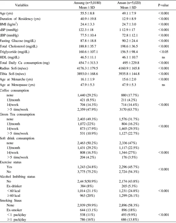
We recruited 10,038 subjects from the two com- munity population; 5,020 urban subjects and 5,018 rural. Demographic characteristics are shown in Table 1. The mean age of the rural subject was 55.5±8.8 that is significantly older in the urban (P＜0.001);

mean age in the urban was 49.1±7.9. Gender distri- bution for urban was very similar (male 50.3% vs female 49.7%) but higher proportionof female subjects (55.4%) was seen in rural area. As shown in table 1, we found significant differences in the many demo- graphic characteristics between the two groups. BMI was significantly higher in the urban (24.7±3 kg/m

²

) than rural region (24.4±3.3 kg/m

²

)(P＜0.01). Mean duration of residence was significantly longer in rural than urban indicating that urban population of more dynamic characteristics. However, other that blood pressures and triglyceride, all other metabolic vari- ables were significantly higher in urban population.

Mean SoS for radius was higher in rural but tibia value was greater in urban population. Mean age at menarche was significantly older in the rural region (16.1±1.9 years) and urban region (15.6±2 years) (P

＜0.001). However, menopause age was not statis-

tically significant different in the two geographic

regions; rural region was 47.9±5.3 years and urban

47.9±5.3 years. Amount of daily calcium intake was

greater in urban population. We also evaluated life

style factors such as drinking habit, smoking and

exercise. There were more urban people drinking and

amount of alcohol intake was also significantly higher

(5)

Table 1. Demographic characteristics

Variables Ansung (n=5,0180) Mean±SD

Ansan (n=5,020)

Mean±SD P-value

Age (yrs)

Duration of Residency (yrs) BMI (kg/m²)

sBP (mmHg) dBP (mmHg)

Fasting Glucose (mg/dL) Total Cholesterol (mg/dL) Triglyceride (mg/dL) HDL (mg/dL)

Total Daily Ca consumption (mg) Radius SoS (m/sec)

Tibia SoS (m/sec) Age at Menarche (yrs) Age at Menopause (yrs)

55.5±8.8 40.9±19.8

24.4±3.3 122.3±18

77.5±10.4 87.8±18.8 188.8±35.7 160.6±107.1

46.5±11.1 454.7±313.3 4176.3±179.5 3893.0±168.6

16.1±1.9 47.9±5.3

49.1±7.9 12.9±8.9 24.7±3.0 1 12.9±17

72.8±12.1 90.2±24.4 198.6±36.5 156.5±98.4 46.1±10.7 495±229.8 4160.9±165.8 3935.8±144.8

15.6±2.0 47.9±5.3

＜0.001

＜0.05 ns

＜0.001

＜0.001 ns Coffee consumption

none 13/month 14/week ＞5 time/week

1,440 (29.2%) 421 (8.5%) 704 (14.3%) 2,359 (47.9%)

880 (17.7%) 211 (4.2%) 714 (14.4%) 3170 (63.7%)

＜0.001

Green Tea consumption none

13/month 14/week ＞5 time/week

2,403 (49.3%) 1,072 (22%)

873 (17.9%) 531 (10.9%)

1,576 (31.7%) 804 (16.2%) 1,465 (29.5%) 1,127 (22.7%)

＜0.001

Soft drink consumption none

13/month 14/week ＞5 time/week

2,463 (50.2%) 1,431 (29.2%) 808 (16.5%) 204 (4.2%)

2,336 (47%) 1,117 (22.5%) 1,344 (27%)

176 (3.5%)

＜0.001

Exercise status Yes No

1,243 (24.8%) 3,775 (75.2%)

2,296 (45.7%)

2,724 (54.3%) ＜0.001

Alcohol Imbibing status No

Ex-drinker ＜60 kcal ≥60 kcal

2,44 5(50.9%) 384 (8%)

1,014 (21.1%) 963 (20%)

2,174 (43.8%) 265 (5.3%) 1,231 (24.8%) 1,299 (26.1%)

＜0.001

Smoking Staus None Ex-smoker ＜1 pack/day ≥1 pack/day

2,939 (59.9%) 644 (13.1%) 538 (11%) 786 (16%)

2,896 (58.3%) 896 (18%) 493 (9.9%) 686 (13.8%)

＜0.001

in the rural area. Coffee intake, carbonated drink, and green tea consumption was also greater in rural area.

There were more smokers but lesser exercise in rural

area. It was very clear that demographic characteristic between the two regions were significantly different.

Since we found significant differences in the mean

(6)

Table 2. Crude rates at tibial

Age Group Sex Ansung Ansan

Osteoporosis n Age-Specific rate Osteoporosis n Age-Specific rate

40～49 M 7 689 0.01 23 1,590 0.014

F 67 856 0.078 54 1,331 0.041

50～59 M 14 658 0.021 8 527 0.015

F 193 788 0.245 91 521 0.175

60～69 M 25 875 0.029 14 272 0.051

F 458 1,101 0.416 130 382 0.34

Total

M 46 2,222 0.021 45 2,389 0.019

F 718 2,745 0.262 275 2,234 0.123

All 764 4,967 0.154 320 4,623 0.069

Table 3. Standardized mortality rate by direct adjustment for tibia

Age Group Sex

Ansung Ansan

Population Age-Specific rate

Estimated

Cases Population Age-Specific rate

Estimated Cases 40～49 M 3,487,210 0.01 34,872 3,487,210 0.014 48,821

F 3,411,518 0.078 266,098 3,411,518 0.041 139,872

50～59 M 2,127,806 0.021 44,683 2,127,806 0.015 31,917

F 2,167,404 0.245 531,013 2,167,404 0.175 379,296

60～69 M 1,422,761 0.029 41,260 1,422,761 0.051 72,561

F 1,729,127 0.416 719,317 1,729,127 0.340 587,903

Total

M 7,037,777 0.017 120,815 7,037,777 0.022 153,299

F 7,308,049 0.208 1,516,428 7,308,049 0.151 1,107,071

All 14,345,826 0.114 1,637,243 14,345,826 0.088 1,260,370

Radius and Tibia SoS lever, we compared prevalence of osteoporosis separately. The crude rate of Tibia osteoporosis for rural area was 15.4% (male=2.1%, female=26.2%), and for urban of 6.9% (male=1.9%, female=12.3%) (Table 2). We found similar rates in male but more than two fold higher female rates were seen in rural area. Moreover, when the rates were further stratified by the age groups (ie., 40, 50, and 60

^th

), we found clear pattern of a linear increments in female subjects. However, increment patterns are milder in male subjects. In females, the magnitude of rates changes was greater in tibia than radius in both regions. The changing patterns clear show a strong

age effects on the prevalence of both tibia and radius

osteoporosis (Tables 2 and 4). There was an evidence

of significant age and gender distribution between the

two regions; we found more female and older subjects

(≥60 years) been recruited in the rural area than

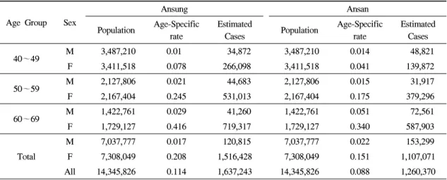
urban. Therefore, we calculated standardized mortality

rates (SMR) by using the direct adjustment to make

direct comparison between the two regions. A shown

in table 3, we found 1.3 times higher rates in urban

male, but 1.4 times higher in rural females. However,

the direct adjustment reduced the rate differences

significantly but still showing 1.3 time higher osteo-

porosis rates in rural population.

(7)

Table 4. Crude rates at radius

Age Group Sex Ansung Ansan

Osteoporosis n Age-Specific rate Osteoporosis n Age-Specific rate

40～49 M 8 686 0.012 19 1,592 0.012

F 6 855 0.007 4 1,338 0.003

50～59 M 14 655 0.021 23 528 0.044

F 51 776 0.066 48 526 0.091

60～69 M 25 865 0.029 15 271 0.055

F 158 1,062 0.149 105 381 0.276

Total

M 47 2,693 0.017 57 2,391 0.024

F 215 2,206 0.097 157 2,245 0.07

All 262 4,899 0.053 214 4,636 0.046

Table 5. Standardized mortality rate by direct adjustment for radius

Age Group Sex

Ansung Ansan

Population Age-Specific rate

Estimated

Cases Population Age-Specific rate

Estimated Cases

40～49 M 3,487,210 0.012 41,847 3,487,210 0.012 41,847

F 3,411,518 0.007 23,881 3,411,518 0.003 10,235

50～59 M 2,127,806 0.021 44,684 2,127,806 0.044 93,623

F 2,167,404 0.066 531,013 2,167,404 0.091 379,296

60～69 M 1,422,761 0.029 143,049 1,422,761 0.055 78,252

F 1,729,127 0.149 257,640 1,729,127 0.276 477,239

Total

M 7,037,777 0.033 229,580 7,037,777 0.03 213,722

F 7,308,049 0.111 812,534 7,308,049 0.119 866,770

All 14,345,826 0.0726 1,042,114 14,345,826 0.075 1,080,492

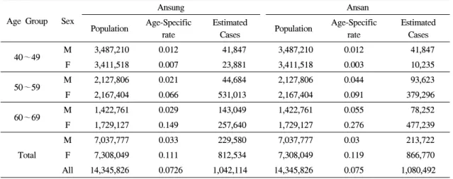
Table 4 shows an overall crude prevalence of radius osteoporosis in the urban was 4.6% and rural with 5.3%. We also observed gender differences, higher rates in urban male (2.4 vs 1.7%) but lower in female

(7% vs 9.7%). However, when SMR was calculated by direct method, differences in both genders were narrowed and found very similar rates, and geographic difference was observed only at tibia.

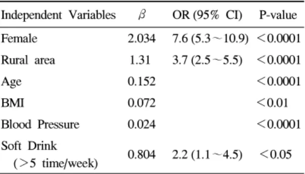
We further evaluated effect of residency on preva- lence of osteoporosis independent of other putative risk factors using multiple logistic regression models.

we found that population living in rural area was 3.3 times (95% CI 2.4～4.7, P＜0.0001) higher risk for

osteoporosis at radius when compared to urban living (Table 6). This relationship existed independent of female gender, age, BMI and blood pressures. Female gender was the strongest independent risk factor for radius osteoporosis. When compared with male gender females are 9.6 time (95% CI 7～13, P＜0.0001) at greater risk for radius osteoporosis. Furthermore, these relationship also persisted at tibia with 3.7 times (95%

CI 2.5～5.5, P＜0.0001) higher risk been living in

Rural area. Similar independent variables were

included in the model along carbonated drink more

than 5 times per week. Female gender was one of the

strongest independent risk factor for tibia osteoporosis.

(8)

Table 6. Multiple logistic regression model for tibia

Independent Variables β OR (95% CI) P-value Female 2.034 7.6 (5.3～10.9) ＜0.0001 Rural area 1.31 3.7 (2.5～5.5) ＜0.0001

Age 0.152 ＜0.0001

BMI 0.072 ＜0.01

Blood Pressure 0.024 ＜0.0001

Soft Drink

(＞5 time/week) 0.804 2.2 (1.1～4.5) ＜0.05

Table 7. Multiple logistic regression model for radius

Independent Variables β OR (95% CI) P-value

Female 2.264 9.6 (7～13) ＜0.0001

Rural area 1.21 3.3 (2.4～4.7) ＜0.0001

Age 0.156 ＜0.0001

BMI 0.064 ＜0.01

Blood Pressure 0.022 ＜0.0001

When compared with male gender females are 7.6 time (95% CI 5.3～10.9, P＜0.0001) at greater risk for tibia osteoporosis. This study demonstrated geographic differences in the prevalence of tibia osteoporosis only (i.e, 1.3 times higher rates in rural area).

Discussion

Osteoporosis is no longer the problematic disease of developed countries. It is affecting developed, develo- ping and as well as under-developing countries in all ethnic groups including young age groups and males.

It is a serious bone metabolic disease and responsible for the majority of non-traumatic collies', spine and hip fractures. Osteoporosis can be prevented if we intervene the risk factors effectively. For better under- standing of the key risk factors for osteoporosis, 1) we need to conduct more population based epide- miologic studies, 2) using standardized diagnostic instrument, finally 3) try to identify the risk factors that could direct and indirectly measure life long exposure to such as living environment. Therefore, in this communitycohort prospective epidemiologic study, we attempt to evaluate residency as the representative risk factor and compared the rate of osteoporosis in two regions within the same population. However, the population based studies have been hampered due to various limitations of available densitometers in the

community; such as high price, high examination costs, availability of bone densitometers in the com- munity, and inaccuracy of the some instruments. Thus far, to overcome aforementioned problems numerous densitometers have been developed and demonstrated reliability of the instrument. Kim et al demonstrated that although the QUS measures different bone properties and measurements are taken at different sites, it is a very useful instrument with a high degree of validity, sensitivity and reliability. The QUS method also demonstrated a significant relationship to predict bone health at other sites such as spine, femur and forearm

²²

. Frost et al. also revealed a positive side of using calcaneal BUA and SOS measurements for an alternative tool for identifying individuals with low bone mass and possible candidates for therapeutic intervention

²³

. Therefore, in this community based population study, we used same QUS method at two different regions to make direct comparison and geographic issue as one of the risk factors for osteo- porosis.

Numerous risk factors such as nutrition, life style,

family history, habitual factors are found to associate

with the rate of osteoporosis. However, these factors

do not predict major percent of osteoporosis and more

risk factors are still remaining to be identified. Thus,

in this study, the goal was to investigate environ-

mental factor .i.e., residential region, as the risk of a

whole. A large number of studies investigated geo-

graphic variations in the level of BMD, osteoporosis,

(9)

and fracture rates. Wu et al. reported racial diffe- rences in BMD reference curves, prevalence, and risks of osteoporosis at various skeletal sites exist among native Chinese, Japanese, and American Caucasian women. The authors reported that there were signi- ficant differences in the peak BMD at various sites among the Chinese, Japanese, and Caucasian women (P＜0.001). In the same study, the average T-scores for BMD loss at various sites in Chinese womenwere higher than those for both Japanese and Caucasian women except at the femoral neck, where the T-scores of Chinese women were exceeded by those of both Japanese and Caucasian women. Estimated from the T-score curve of BMD loss, the age of osteoporosis occurrence at the femoral neck in Chinese women was about 10 years later than that in Japanese or Caucasian women; at the AP spine, Chinese women were similar to Japanese women; at the other sites, the age for occurrence of osteoporosis in Chinese women was about 5～15 years earlier than that in either Japanese or Caucasian women

²⁴

. This study clearly demonstrated ethnic difference in BMD levels and osteoporosis.

The report from Hong Kong revealed that in- creasing hip fracture rates have been attributed toincreasing urbanization

²⁵

. Moreover, differences in rural and urban hip fracture rates have been reported between communities in North America, Asia and Scandinavia. In most of the studies, lower fracture rates were reported in rural communities and increa- sing hip fracture rates in Asian have been attributed to increasing urbanization

^25～29

. However, Sanders et al. reported 32% lower hip fractures among rural than urban residents

²⁶

. These geographic differences in the fracture rates might be relate to the rate of osteo- porosis. Although, there are limited number of epide- miologic studies directly compare the geographic differences within the same population, an existing literature showed a higher rates of osteoporosis in urban area.

Vu et al. conducted a population-based, cross- sectional survey to determine the prevalence of osteoporosis and related factors in Vietnamese adult women by using quantitative ultrasound at the heel bone (calcaneus). A total of 2,232 adult women aged

≥20 years were studied and found the crude prevalence of osteoporosis 15.4%; after adjustment for age, it was 9.0%. The authors also found higher osteoporosis rates in the urban areas compared with the rural areas

³⁰

. Yang et al. also reported higher mean BUA levels in urban area subjects when compare to that of rural area subjects in almost all age-strata

³¹

. However, our study showed no differences in males but higher tibia osteoporosis rates in women living in rural area when therate was adjusted by the direct method. Findings from this study are controversial to the other previous reports from Asia. These differences might be related to: 1) rate of osteoporosis are specific to measurement sites, 2) other unknown risk factors are involved in geographic factors.

In conclusion, this is the first study to investigate geographic differences in the rate of osteoporosis in Korea using standardized method. The results indicate that the most important predictors for tibia and radius osteoporosis were age, gender, blood pressure, BMI, and rural dwelling. Thus, we suggest that rural dwelling women should be closely monitored for osteoporosis, specifically tibia after 50 years of age.

Abstract

Objectives: To investigate geographic differences in the prevalence of tibia and radius osteoporosis in a community-based cohort.

Methods: In this community cohort prospective

study, a total of 10,038, 40～69 years old subjects

(male=4,762, female=5,276) from both urban and

rural regions were recruited; all of them underwent

Quantitative Ultrasound (QUS) measurements at Radius

(10)

and Tibia to diagnose osteoporosis. WHO criteria were used to interpret the QUS results for diagnose of osteoporosis. Standardized method including QUS measuring device and questionnaire was used by the trained researchers.

Results: The mean age of the rural subject was 55.5±8.8 that is significantly older in the urban region 49.1±7.9 (P＜0.001). Gender distribution in urban was very similar (male 50.3% vs female 49.7%) but higher proportion of female subject (55.4%) in rural. Many demographic characteristics were signifi- cantly different between the two groups; BMI was higher in urban (24.7±3 kg/m

²

vs 24.4±3.3 k/m

²

) (P

＜0.01), mean duration of residence was significantly longer in rural (41 years vs 13 years). Exception of blood pressures and triglyceride, all other metabolic variables were significantly higher in urban popula- tion. Mean SoS for radius was higher in rural but tibia value was higher in urban population. Mean age at menarche was significantly older in rural (16.1± .9 years vs 15.6±2 years) (P＜0.001). Amount of daily calcium intake, alcohol intake, coffee, carbonated drink, and green tea consumption was greater in urban, but more smokers and lesser exercise in rural subjects. We calculated standardized mortality rates by using the direct adjustment to make direct comparison between the two regions. At tibia, osteoporosis in rural was 11.4% (male=1.7%, female=20.8%) and urban 8.8% (male=2.2%, female=15.1%). At radius, osteoporosis in rural was 7.3% (male=3.3%, female=

11.1%) and urban 7.5% (male=3%, female=11.9%).

Multiple logistic regression analysis revealed that rural dwelling was 3.3 times (95% CI 2.4～4.7, P＜0.0001) higher risk for osteoporosis at radius when compared to urban independent of female gender, age, BMI and blood pressures. These relationship also persisted at Tibia with 3.7 times (95% CI 2.5～5.5, P＜0.0001) higher risk in rural dwelling. Similar independent variables were persisted in addition to carbonated drink (＞ 5 times per week).

Conclusion: This is study results indicate that the most important predictors for tibia and radius osteo- porosis were age, gender, blood pressure, BMI, and rural dwelling. We suggest that rural dwelling women should be closely monitored for osteoporosis, specifi- cally tibia after 50 years of age.

Key Words: Urban-rural, Prevalence, Osteoporosis, Korea

Reference

1. Sexton P, Sexton T. Excess coronary mortality among Australian men and women living outside the capital statistical division. Med J Aust 2000;

172:370-4.

2. Schootman M, Fuortes L. Breast and cervical carcinoma: the correlation of activity limitations and rurality with screening, disease incidence, and mortality. Cancer 1999;86:1087-94.

3. Howe H, Johnson T, Lehnherr M. Patterns of breast cancer treatment: a comparison of a rural population with an urban population and a community clinical oncology program sample.

Cancer Control 1995;2:113-20.

4. Ross PD. Prediction of fracture risk. II. Other risk factors. Am J Med Sci 1996;312:260-9.

5. Cummings SR, Black DM, Nevitt MC, Browner W, Cauley J, Ensrud K, et al. Bone density at various sites for prediction of hip fractures. The Study of Osteoporotic Fractures Research Group.

Lancet 1993;9:72-75.

6. Cummings SR, Kelsey JL, Newitt MC, O'Dowd KJ. Epidemiology of osteoporotic fractures. Epide- miol Rev 1985;7:178-208

7. Obrant KJ, Bengner U, Johnell O, Nilsson BE, Sernbo I, et al. Increasing age-adjusted risk of fragility fractures:a sign of increasing osteoporosis in successive generations? Calcif Tissue Int 1989;

44:157-167.

8. Kanis JA, Pitt FA. The epidemiology of osteo-

(11)

porosis. Bone 1992;13:S7-S15.

9. Raisz LG, Prestwood KM. Epidemiology and pathogenesis of osteoporosis. Clin Cornerstone 2000;2:1-10.

10. Lau E. Epidemiology of Osteoporosis in Urba- nized Asian Population. Osteoporosis Int 1997;

7(Suppl. 3):S91-95.

11. Kanis JA, Pitt FA. Epidemiology of osteoporosis.

Bone 1992;13(Suppl. 1):S7-15.

12. Rowe S, Jung S, Lee J. Epidemiology of Osteo- porosis in Korea. Osteoporosis Int 1997;7(Suppl.

3):S88-90.

13. Kaneki M, Hedges SJ, Hosoi T, Fujiwara S, Lyons A, Crean SJ, et al. Japanese fermented soybean food as the major determinant of the large geographic difference in circulating levels of vitamin K2: possible implications for hip-fracture risk. Nutrition 2001;17:315-21.

14. Lunt M, Felsenberg D, Adams J, Benevolenskaya L, Cannata J, Dequeker J, et al. Population-based geographic variations in DXA bone density in Europe: the EVOS Study. European Vertebral Osteoporosis. Osteoporos Int 1997;7:175-89.

15. Weaver CM.The growing years and prevention of osteoporosis in later life. Proc Nutr Soc 2000;

59:303-6.

16. Santora AC 2nd. Role of nutrition and exercise in osteoporosis. Am J Med 1987;82(1B):73-9.

17. Shin C, Abbott RD, Lee H, Kim J, Kimm K.

Prevalence and correlates of orthostatic hypoten- sion in middle-aged men and women in Korea:

the Korean Health and Genome Study. J Hum Hypertens 2004;18:717-23.

18. Gray DS, Bray GA, Gemayel N, Kaplan K. Effect of obesity on bioelectrical impedance. Am J Clin Nutr 1989;50:255-60.

19. Vache C, Rousset P, Gachon P, Gachon AM, Morio B, Boulier A, et al. Bioelectrical impedance analysis measurements of total body water and extracellular water in healthy elderly subjects. Int

J Obes Relat Metab Disord 1998;22:537-543.

20. Friedewald WT, Levy RI, Fredrickson DS, Esti- mation of the concentration of low-density lipo- protein cholesterol in plasma, without use of the preparative ultracentrifuge. Clin Chem 1972;18:

499-502.

21. The World Health Organization (WHO) Study Group 1994 Assessment of fracture risk and its application to screening for postmenopausal osteo- porosis. Technical Report Series 843, WHO, Geneva, Switzerland.

22. Kim KI, Han IK, Kim H, Cho NH. How reliable is the ultrasound densitometer for community screening to diagnose osteoporosis in spine, femur, and forearm? J Clin Densitom 2001;4:159-65.

23. Frost ML, Blake GM, Fogelman I. Quantitative ultrasound and bone mineral density are equally strongly associated with risk factors for osteopo- rosis. J Bone Miner Res 2001;16:406-16.

24. Wu XP, Liao EY, Huang G, Dai RC, Zhang HA comparison study of the reference curves of bone mineral density at different skeletal sites in native Chinese, Japanese, and American Caucasian women.

Calcif Tissue Int 2003;73:122-32.

25. Lau EMC. The epidemiology of hip fracture in Asia: an update. Osteoporosis Int 1996;6(Suppl.

3):s19-23.

26. Sanders KM, Nicholsen GC, Ugoni AM, Seeman E, Pasco JA, Kotowicz MA. Fracture rates lower in rural than urban communities: the Geelong Osteoporosis Study. J Epidemiol Comm Health 2002;56:466-70.

27. Falch JA. Kaastad TS, Bohler G, Espeland J, Sundsvold OJ. Secular inrease and geographical differences in hip fracture incidence in Norway.

Bone 1993;14:643-5.

28. Mannius S, Mellstrom D, Oden A, Rundgren A,

Zetterberg C. Incidence of hip fracture in western

Sweden 1974-1982. Comparison of rural and

urban populations. Acta Ortho Scand 1987;58:

(12)