609
ondary motion sets in, starting at a certain time. For Re≥ ReG the dimensionless critical time to mark the onset of vortex instabilities, τc, is here presented as a function of the Reynolds number Re and the radius ratio η. For the wide gap case of small η, the transient instability is possible in the range of ReG≤ Re ≤ ReS. It is found that the predicted τc-value is much smaller than experimental detection time of first observable secondary motion. It seems evident that small distur- bances initiated at τc require some growth period until they are detected experimentally.
Key words: Taylor-Görtler Vortex, Energy Method, Relative Stability
1. Introduction
In flows along concavely curved walls, the destabilizing action of centrifugal forces can produce an instability motion in form of sta- tionary vortices. This instability is analogous to that of Taylor-Gör- tler vortices. The impulsive spin-down of initial rigid-body flow between two coaxial cylinders evolves into a secondary flow pattern which consists of a series of Taylor-like vortices. In this transient boundary-layer system the critical time tc to mark the onset of sec- ondary motion becomes an important question. In this connection the instability problem of decelerating circular flow has attracted interests.
Tillman[1] first investigated experimentally the onset of instabil- ity in the flow system of spin-down from solid-body rotation of coaxial cylinders filled with liquid suddenly brought to rest. The ana- lytical difficulties involved in the application of conventional stabil- ity theory to this kind of transient flow has been considered[2] and the related instability analysis has been conducted by using the strong and the marginal stability criteria[3-5]. The strong stability criterion pursued the stability bounds in terms of time interval where the kinetic energy of disturbances starts to increase. The marginal stability criterion which relaxes the strong one shifts the stability bounds to a more stable direction. However it has been faced with mathematical difficulties. These models consider some finite, initial disturbances and trace the temporal growth of their kinetic energy.
In the present study, we will analyze the onset of Taylor-Görtler
vortices in impulsively decelerating transient circular flow between coaxial two cylinders. This problem was already analyzed using the aforementioned models. We will relax the strong stability criterion by introducing the relative one, which has been used in the various problems[6-10]. The new stability equations will be derived for the whole time region and the resulting predictions will be compared with available experimental and theoretical results. Also, the effects of stability criteria on the critical conditions will be examined. Since the present system is a rather simple one, the present results will be helpful for comparison among available models.
2. Theoretical Analysis
2-1. Governing Equations
The system considered here is a Newtonian fluid confined between the cylinders of radii Ri and Ro. Let the axis of the cylinders be along the vertical z'-axis under the cylindrical coordinates (r', θ, z') and the corresponding velocities be U, V and W. The entire fluid/cylinder system is assumed to be in a state of rigid-body rotation with angular velocity Ω. Starting from time t = 0, the outer cylinder is impul- sively stopped. The ensuing unsteady flow is known as spin-decay one. The schematic diagram of the present system is shown in Fig. 1.
Such transient circular flow is known to be subjected to instability in form of Taylor-Görtler vortices and the governing equations of the flow field are expressed as
, (1)
, (2)
where U, P, ν and ρ represent the velocity vector, the dynamic pressure, the kinematic viscosity and the density, respectively.
∇ U⋅ =0
∂t∂ ----+U ∇⋅
⎩ ⎭
⎨ ⎬
⎧ ⎫U 1
ρ---
– ∇P ν∇+ 2U
†To whom correspondence should be addressed. = E-mail: [email protected]
This is an Open-Access article distributed under the terms of the Creative Com- mons Attribution Non-Commercial License (http://creativecommons.org/licenses/by- nc/3.0) which permits unrestricted non-commercial use, distribution, and reproduc- tion in any medium, provided the original work is properly cited.
The primary-velocity field is represented for the case of constant physical properties:
, (3)
with the following initial and boundary conditions,
, and . (4)
where and . Neitzel [4] obtained the fol- lowing analytical, exact solution as
, (5a)
where
. (5b)
In the above J and Y are Bessel functions of the first and the sec- ond kind, respectively, r = (r' - Ri)/d, η = Ri/Ro and τ = νt/d2, here d = Ro- Ri. (λi, ci) are the roots of the equations
(5c) and
(5b) where
(5d) For the limiting case of η→1, i.e. very narrow gap, the curvature effects can be negligible and the above velocity profile can be represented by using the complementary error function as
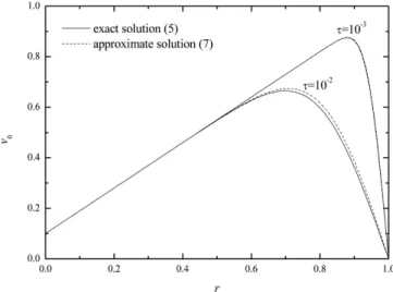
for η→1. (6) For small time, the velocity profiles of Eqs. (5) and (6) can be approximated as
for τ→0. (7)
The instantaneous base flow profile is shown in Fig. 2. As shown in this figure for τ ≤ 10-3, the deep-pool solution (7) approximates the exact solution (5) quite well. To reduce computation time, Eq. (7) is used in stability analysis for the region of τ ≤ 10-3. From this profile the centrifugal instability near the outer cylinder wall can be expected based on the Rayleigh criterion for the inviscid flow[5]. However, sophisticated stability analysis is required to obtain stability limit since present system is time-dependent and viscous.
2-2. Energy Method
Following the work of Serrin[11] and Neitzel[4], the energy iden- tity is written as
, (8)
where , , φ = (1/r −∂/∂r)ν0 and .
Here u(=U/Vi) is the dimensionless velocity vector, Re(=Vid/ν) is the Reynolds number and represents the average over the system.
The conventional energy method determines the critical times to mark the onset of secondary motion at which E is the minimum, i.e.
at τ = τs. (9)
This condition is known as the strong stability criterion[2]. Neitzel[4]
relaxed this strong stability criterion by considering the growth of the disturbance kinetic energy. For a given Re, the marginal stability τm is determined implicitly from the condition of
, (10)
∂V0
---∂t =νD′D*′ V0
V0(0 r, ′) r′Ω= V0(t R, i) R= iΩ V0(t R, o) 0= D′ ∂/∂r′= D*′ D′ 1/= + r′
v0( )τ r, V0 RoΩ --- η2
1+η
( )
---
– r 1
1–η ( )2 ---
⎝ – ⎠
⎛ ⎞
= =
+ 1( –η) kn[J1( ) cλir + iY1( )λir ]exp λ(– i2τ)
i 1=
∑
∞kn 2Z0 λi
1–η ---
⎝ ⎠
⎛ ⎞ λi η2Z02 λiη 1–η ---
⎝ ⎠
⎛ ⎞ Z02 λi
1–η ---
⎝ ⎠
⎛ ⎞
⎩ – ⎭
⎨ ⎬
⎧ ⎫–1
=
Z1(λiη/ 1 η( – )) 0=
Z1(λi/ 1( –η)) 0=
Zk≡Jk+ciYk
v0( ) 1τ r, erfc n ---τ 1 r–
2 τ ---
⎝ + ⎠
⎛ ⎞ erfc n 1+
---τ 1 r– 2 τ ---
⎝ – ⎠
⎛ ⎞
⎩ – ⎭
⎨ ⎬
⎧ ⎫
n 0=
∑
∞–
=
v0( ) 1 1 rτ r, ( – ) 1 η( – ) erfc– 1 r– 2 τ --- –
=
dE dτ
---=ReI D–
E=〈u u⋅ 〉/2 I=〈uνφ〉 D=〈∇u:∇u〉
〈 〉·
dE dτ ---=0
σ τ′( ) τ′d
0 τm
∫
=0Fig. 1. Top view of the system considered here. Fig. 2. Primary-velocity profiles for η = 0.1.
tive stability concept: the temporal growth rate of the kinetic energy of the disturbance velocity should exceed that of the base velocity at the onset condition of secondary motion. This stability criterion was proposed by Chen et al.[2], and applied into the various problems by Kim et al.[6-10]. In the relative stability model the critical time τr is determined, based on a most dangerous mode of instability:
at , (13)
where , dτ and E0 is the basic
centrifugal potential energy, i.e. E0= . The above criterion means that secondary motion sets in at τr when the growth rates of the energy of disturbance and base quantity are the same. In the strong and marginal stability criterion, only the decay or growth of disturbance quantity is taken into account. Based on Eqs. (8) and (13), the relaxed energy identity for the relative stability model becomes
. (14)
Now, the relative stability limit is given by
. (15)
Under the normal mode analysis the typical axisymmetric distur- bances, which have been observed experimentally[1,13,14] and known as the energetically most unstable mode[5], are well rep- resented by
, (16a)
w1= w' sin az, (16b)
where a is the dimensionless wavenumber representing the peri- odicity in the z'-direction, z = z'/d and the primed quantities rep- resenting disturbance amplitudes are a function of r and τ. Here we assume the infinitely long cylinder and neglect the endwalls effects. Then this maximum problem can be solved by the varia- tional technique[11]. By eliminating the Lagrage multiplier term with the aid of continuity equation, the Euler-Lagrange equations for the relative stability model are obtained:
, (20)
where f(η) = {1/4 − 3η2/4−η4lnη}/{(1+η)(1−η)3}, and bi and ci
are bi(λi, η) = , and =
.
For the limiting case of η→1, σ0 is obtained from Eq. (6) as
. (21)
For the case of τ→∞, the above stability equations with σ0= 0 degenerate into the strong stability formulation. And, for the limit- ing case of τ→0, based on the velocity profile of Eq. (7), it is found that σ0= (1/E0)(dE0/dτ) = 1/2τ and therefore, the terms containing σ0/2 should be changed as 1/4τ.
2-3. Solution Method
The stability equations (17)-(19) are solved by employing the shooting method[15]. In order to integrate these stability equations the proper values of ∂2u'/∂r2, ∂3u'/∂r3 and ∂ν'/∂r at r = 1 are assumed for a given τ and a. Since the stability equations and their boundary conditions are all homogeneous, the value of ∂3u'/∂r3 at r = 1 can be assigned arbitrarily and the value of the parameter Re is assumed.
This procedure can be understood easily by taking into account the characteristics of eigenvalue problems. After all the values at r = 1 are provided, this eigenvalue problem can be proceeded numeri- cally. Integration is performed from r = 1 to r = 0 with the fourth order Runge-Kutta-Gill method. If the guessed values of Re, ∂3u'/∂r3 and
∂v'/∂r at r = 1 are correct, u', ∂u'/∂r and ν' will vanish at r = 0. The minimum Re-value is found in the plot of Re vs. a.
3. Results and Discussion
The stability conditions obtained from the present relative and the σ1=σ0 τ τ= r
σ1=(1/E) dE/dτ( ) σ0=(1/E0) dE( 0/dτ) ν0( ) ντ r, – 0(0 r, )
{ }2
〈 〉/2
σ0E=ReI D–
1
Re--- max I D+σ0E ---
=
u1, ,ν1 p1
( )=(u′ ν′ p′, , )cos az
σ0 2λi
– exp
i 0
∑
= (–λiτ) b{ i exp(–λiτ) c+ i}f( )η exp
i 1=
∑
∞ (–λi2τ) b{ i exp(–λ2iτ) 2c+ i}+
---
=
ki2
---2 Z1′ λi 1–η ---
⎝ ⎠
⎛ ⎞
⎝ ⎠
⎛ ⎞2 ηZ1′ ηλi 1–η ---
⎝ ⎠
⎛ ⎞
⎝ ⎠
⎛ ⎞2
⎩ – ⎭
⎨ ⎬
⎧ ⎫
ci(λi,η) ki
λi
----Z0 λi 1–η ---
⎝ ⎠
⎛ ⎞
σ0
8 exp
i 0=
∑
∞ (–n2π2τ) 1 exp n{ – (– 2π2τ)}1/3 exp
n 1=
∑
∞– (–n2π2τ)/ nπ( )2{2 exp– (–n2π2τ)} ---
=
conventional strong stability model are illustrated in Fig. 3. It is known that the approximation (8) produces the same values as those from Eq. (5) as time decreases. As discussed below Eq. (19), the present relative stability model yields the strong stability limit as τ→∞. For the limiting case of τ→∞, the stability equations (15)-(17) are reduced to
, (22)
, (23) under the very narrow gap condition, i.e. η→1, where φ→1 and σ0→0 from Eqs. (5) and (19), respectively. The proper boundary conditions are
at r = 0 and 1. (24)
According to the calculation of Chandrasekhar’s[16], the critical condition is (ReS/2)2= 1,708 and ac= 3.117, i.e. ReS= 82.66 for η→1, here ReS is the steady state critical Reynolds number. And, for the another limiting case of small τ, the critical time to mark the onset of a fastest growing instability decreases with increasing Re. Based on the base velocity field given in Eq. (7), they approach :
as τ→0, (25a)
for the relative stability, and
as τ→0, (25b)
for the strong stability, as are illustrated in Fig. 3.
For the case of a rather wide gap η ≤ 0.5, there exists the subcriti- cal region where the global minimum of the critical Reynolds num- ber, ReG is lower than ReS. In the range of ReG≤ Re ≤ ReS, the instability is transient and decays out as τ→τf, here τf is the decay time from which the instability cannot be guaranteed. Therefore, for the region of Re > ReG the curves in Fig. 3 correspond to the decay
time. Neitzel[4] and Chen and Neitzel[5] analyzed this problem by employing the marginal stability criterion. As shown in Fig. 4, their marginal stability results shift the strong stability curve to the more stable direction. However, they found the stability limits for the lim- ited range. For the limiting case of η→0, the system is uncondition- ally stable and all instabilities are transient, i.e. all instabilities should be disappeared at a certain time. Even though τf has been predicted for the case of ReG< ReS, it has not been determined experimentally even for the asymtoptically unconditionally-stable case of η→0.
For the case of η = 0.5 the above results are compared with the predictions in Fig. 4. Neitzel’s[4] marginal stability gives slightly more stable results than the present relative stability ones. Following the Neitzel’s[4] idea, we have retried to find τm. First, for a given Re we found σ which satisfys Eq. (11) and constructed the relationship of σ vs. τ by employing a regression analysis. As shonwn in Fig. 5, the regression equation σr(τ) represents the calculated results quite well. Then, the marginal stability time τm is obtained by integrating the regression equation σr(τ) numerically. For the region of Re ≥ 150, 1
2---a2Reν′
– d2
dr2 --- a– 2
⎩ ⎭
⎨ ⎬
⎧ ⎫
u′ 0
= =
1
2---Reu′ d2 dr2 --- a– 2
⎩ ⎭
⎨ ⎬
⎧ ⎫ν′ 0
= =
u′ ∂u′ ---∂r ν′ 0
= = =
τr=389.27Re–2
τs=223.80Re–2
Fig. 3. Characteristic stability curves in the Re-τ diagram. Fig. 4. Comparison among predictions for η = 0.5.
Fig. 5. Comparison of calculated growth rate with its regression func- tion.
the present τm reconstructs Neitzel’s [4] τm. However, for the region of Re < 110, we cannot find τm satisfying Eq. (10). The integration given in Eq. (10) based on the present σr(τ) is always negative for Re< 110, i.e., ReG,m= 110 for the case of η = 0.5 under the marginal stability concept. The present ReG,m is slightly higher than Chen and Neitzel’s[5] global minumum Reynolds number, ReG,m= 102. This minor difference may be come from the method to calculate the defi- nite integral given in Eq. (10). To calculate that integral, Neitzel[4]
used 3-points Gausse-Legendre quadrature which gives exact defi- nite integal value only for a polynomial equation of the 2nd degree.
The present ReG,m is nearly same as the global minumum Reynolds number based on the relative stability concept ReG,r= 109.
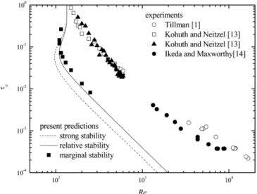
The above results are compared with the available experimental data in Fig. 6. By using the suspended particle Tillman[1] visualized Taylor-Görtler vortex motion for the case of η = 0.625. Later, Kohuth and Neitzel[13] determined the onset time systematically by a photo- diode array and visual observations for the experimental set-up of η = 0.5. Ikeda and Maxworthy[14] visualized the onset of vortex by adding aluminum flake into water placed between two coaxial cylin- ders of η = 0.464. As expected, none of the above stability criteria predict the onset time observed experimentally, as shown in Fig. 6.
This may be caused by several factors. The time for disturbances to grow to finite amplitude before being observed seems to be a major one. Furthermore, the transient stability region was not observed in all the experiments, as mentioned above.
4. Conclusions
The onset of a fastest growing, axisymmetric instability in tran- sient spin-down flow has been investigated theoretically. The strong stability results give the lower bounds on the stability limits, and the present relaxation of the relative instability shifts the stability limit to
1. Tillman, W., “Development of Turbulence during the Build-Up of a Boundary Layer at a Concave Wall,” Phys. Fluids, Supp. 10, S108(1967).
2. Chen, J.-C., Neitzel, G. P. and Jankowski, D. F., “The Influence of Initial Condition on the Linear Stability of Time-Dependent Circular Couette Flow,” Phys. Fluids, 28, 749(1985).
3. Neitzel, G. P. and Davis, S. H., “Energy Stability Theory of Deceler- ating Swirl Flows,” Phys. Fluids, 23, 432(1980).
4. Neitzel, G. P., “Marginal Stability of Impulsively Initiated Couette Flow and Spin-Decay,” Phys. Fluids, 25, 226(1982).
5. Chen, J.-C. and Neitzel, G. P., “Strong Stability of Impulsively Initiated Couette Flow for Both Axisymetric and Non-axisymetric Disturbances,” J. Appl. Mech., 49, 691(1982).
6. Kim, M. C. and Choi, C. K., “Relaxed Energy Stability Analysis on the Onset of Buoyancy-Driven Instability in the Horizontal Porous Layer,” Phys. Fluids, 19, 088103(2007).
7. Kim, M. C., Choi, C. K., Yoon, D. Y. and Chung, T. J., “Onset of Marangoni Convection in a Horizontal Fluid Layer Experi- encing Evaporative Cooling,” I&EC Res., 46, 5775(2007).
8. Kim, M. C. and Choi, C. K., “Analysis of Onset of Soret-Driven Convection by the Energy Method,” Phys. Rev. E, 76, 036302(2007).
9. Kim, M. C., Choi, C. K. and Yoon, D.-Y., “Relaxation on the Energy Method for the Transient Rayleigh-Bénard Convection,”
Phys. Lett. A, 372, 4709(2008).
10. Kim, M. C., “Relative Energy Stability Analysis on the Onset of Taylor-Görtler Vortices in Impulsively Accelerating Couette Flow,”
Korean J. Chem. Eng., 31, 2145-2150(2014).
11. Serrin, J., “On the Stability of Viscous fluid Motions,” Arch. Rat.
Mech. Anal., 3, 1(1959).
12. Gumerman, R. J. and Homsy, G. M., “The Stability of Uniformly Accelerated Flows with Application to Convection Driven by Surface Tension,” J. Fluid Mech., 68, 191(1975).
13. Kohuth, K. R. and Neitzel, G. P., “Experiments on the Stability of an Impulsively-Initiated Circular Couette Flow,” Exp. Fluids, 6, 199(1988).
14. Ikeda, E. and Maxworthy, T., “A Note on the Effects of Polymer Additive on the Formation of Goetler Vortices in a Unsteady Flow,” Phys. Fluids A, 2, 1903(1990).
15. Hwang, I. G., “Characteristics and Stability of Compositional Convection in Binary Solidification with a Constant Solidifica- tion Velocity,” Korean Chem. Eng. Res., 52, 199-204(2014).
16. Chandrasekhar, S., Hydrodynamic and Hydromagnetic Stability, Oxford University Press, Oxford(1961).
Fig. 6. Comparison of predictions η = 0.5 with experimental data:
○, η= 0.625 (Tilman[1]); □, η= 0.5 (visual observation, Kohuth and Neitzel[13]); ▲, η = 0.5 (photo diode array, Kohuth and Neitzel[13]); ●, η = 0.464 (Ikeda and Maxworthy[14]).