ISSN 2234-8352 (Online) J. Korean Soc. of Marine Engineering (JKOSME)
https://doi.org/10.5916/jkosme.2016.40.10.935 Original Paper
This is an Open Access article distributed under the terms of the Creative Commons Attribution Non-Commercial License (http://creativecommons.org/licenses/by-nc/3.0), which permits
†Corresponding Author (ORCID: http://orcid.org/0000-0002-2636-9135): Faculty of Mechanical Engineering and Marine Technology, University of Rostock, Albert-Einstein-Strasse 2, 18059 Rostock, Germany, E-mail: [email protected], Tel: +49-381- 498-9231
1 Graduate school, Faculty of Mechanical Engineering and Marine Technology, University of Rostock, E-mail: [email protected], Tel: +49-173-971-7115
2 ISSIMS Institute, Hochschule Wismar, University of Applied Sciences, Technology, Business and Design, E-mail: [email protected], Tel: +49-381-498-5981
A study on hydrodynamic coefficients estimation of modelling ship using system identification method
Dae-Won Kim1 ․ Knud Benedict2 ․ Mathias Paschen†
(Received December 1, 2016; Revised December 28, 2016;Accepted December 29, 2016)
Abstract: Predicting and evaluating ship manoeuvring characteristics are very important not only for the design stage, but also for the existing vessels. There are several ways to predict ship’s manoeuvrability and most of them are highly connected with the estimation of hydrodynamic coefficients. This paper presents a new estimation method using the system identification with mathematical algorithms for estimating hydrodynamic coefficient in the ship’s mathematical model. Specifically a double ended ferry which equips four azimuth propulsion systems were chosen as benchmark ship and a set of benchmark data which is gen- erated in the fast time simulation software was provided to conduct mathematical optimization process. Also the initial values for the optimization were borrowed from the empirical regression formulas of the simulation software of Rheinmetall Defence ship simulator. Therefore the newly suggested mathematical optimization algorithm gave a successful result for estimation hydro- dynamic coefficients. Proper optimization conditions of the objective function and constraints were also verified during the study.
Keywords: Mathematical optimization, Ship manoeuvrability, System identification, Hydrodynamic coefficients, Ship modelling
1. Introduction
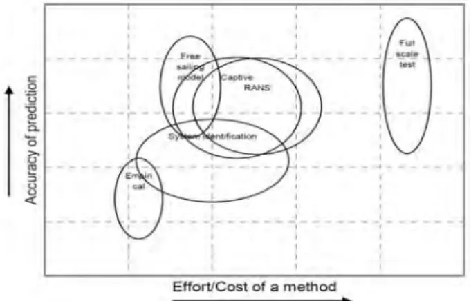
Mathematical modelling is one of the important part to pre- dict ship’s manoeuvrability. Especially for the submerged part of the hull, the forces and moments acting on the hull can be presented by hydrodynamic coefficients. As shown in Figure 1, International Towing Tank Conference (ITTC) summarized dif- ferent methods to estimate hydrodynamic coefficients for the ship’s manoeuvrability[1]. Figure 2 shows that each method has its own accuracy to effort/cost characteristics and Captive model test and Computational Fluid Dynamics (CFD) method are common at design stage[2][3]. These methods are the most reliable source of hydrodynamic coefficients excluding full scale trials, but the relatively high cost and calculation time are required than empirical method and system identification.
This paper examines a new estimation method which is based on the system identification method with full scale sea trial data. This method estimates the hydrodynamic coefficients in a ship’s mathematical model by using mathematical opti- mization algorithm. The algorithm conducts manoeuvring sim- ulation and compares with benchmark data, such as sea trial
data, at every iteration and it provides updated target variables to be optimized.
Various ideas on the system identification has been studied with the progress of computational calculation. Abkowitz [4]
conducted full scale sea trial and firstly applied Extended Kalman Filter (EKF) and Rhee et al. [5] and Zhang et al. [6]
applied System Based (SB) free running tests with the EKF algorithm. Tran et al. [7] introduced SQP and BFGS algo- rithms to get optimal results.
As a preliminary study, a set of simulation result, which used manually tuned double ended ferry ship model corre- sponding to sea trial data, is selected as a benchmark data to be optimized. The Interior-point algorithm optimizes four line- ar hull coefficients and presents optimization results and corre- sponding simulation results.
This paper presents a system identification method based on a new optimization algorithm and its optimization results.
Comparison among the benchmark data, the initial condition of the optimization process and finally tuned data are also pre- sented in this paper.
Figure 1: Overview of manoeuvring prediction methods
Figure 2: Effort/cost versus accuracy of manoeuvring pre- diction methods
2. Ship modelling and benchmark data
2.1 Mathematical model3-Degrees-of-Freedom (DOF) of the ship-fixed and earth-fixed coordinate systems are adopted in this study as shown in Figure 3 [8]. The plane and the
plane lie on the undisturbed free surface, with the axis pointing in the direction of the original heading of the ship, whereas the axis and the axis point downwards vertically. The angle between the directions of the axis and the axis is defined as the heading angle, .
Figure 3: Coordinate system of the vessel
In the simulation of optimization process, mathematical model of Rheinmetall Defence simulator is used to predict ship’s manoeuvrability. When a ship is considered as a mas- sive and rigid body, forces and moment acting on the hull and on the ship-fixed coordinate system on the ship’s center of gravity can be described as Equation (1), according to the Newtonian law of motion.
∙
(1)
Forces and moment of the model are consisted with multi- ple modules as Equation (2): hull, propeller, rudder and other external forces and moments. The external factors are not con- sidered in this study.
(2)
Equation (3) shows the composition of the hydrodynamic forces and moment acting on the hull. In this model, the em- pirical regression formulas of Norrbin[9] and Clarke [10] are applied to calculate the initial hydrodynamic coefficients.
Each hydrodynamic coefficients can be expressed the function of ship’s main dimension as Equation (4): length, beam, draught and displacement of the ship. and are non-linear components of sway force and yaw moment. These non-linear components are dependent on the position of the ship’s turning point.
′ ′ ′ ′ ′ ′
′ ′ ′ ′ ′ ′
′ ′ ′ ′ ′ ′
(3)
′ ′ ′ ′
∆ (4)2.2 Benchmark data
Motor ferry ‘Prins Richard’ is adopted as a benchmark ves- sel to conduct optimization trials and Figure 4 shows the vessel. This RoPax (Roll-on Roll-off Passenger) and on-board railway vessel offers liner service between Puttgarden, Germany and Rødby, Denmark. It applies the ‘double-ended ferry’ structure, which has a specific hull form and a pro- pulsion system, allowing ahead and astern manoeuvring with- out turning the vessel. These hull forms can save manoeuvring time or berthing in the harbour. Due to its specific character, the identical shapes of the bow and stern, the term “astern ma- noeuvre” does not exist for this type of vessel. They are typi-
cally on short crossing routes, which have confined ferry ter- minals and shallow channel conditions [11].
Figure 4: M/F Prins Richard
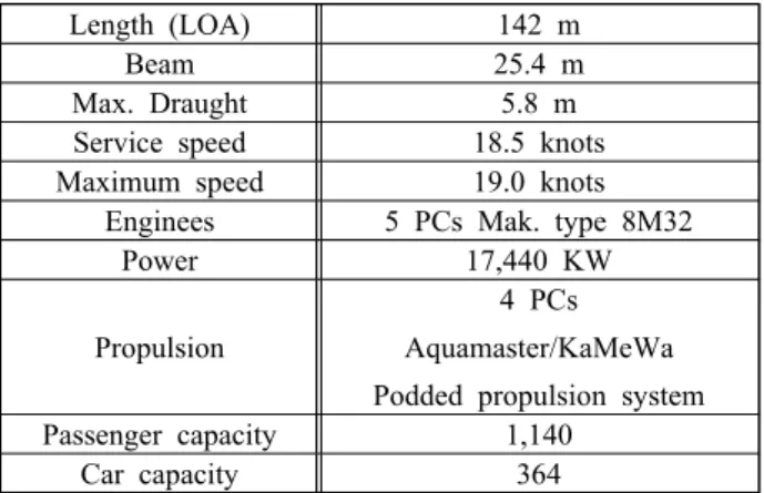
As shown in Table 1, the technical table of the vessel, this ferry equips two pairs of podded contra-rotating propulsion units, which are combined systems for the steering and pro- pulsion modules.
The benchmark data of the optimization process is provided by the simulation software, programmed by MATLAB/
Simulink. Technical data and model data of the benchmark ship is brought from Maritime Simulation Center Warnemünde (MSCW) and ISSIMS Institute of Hochschule Wismar in Germany.
Length (LOA) 142 m
Beam 25.4 m
Max. Draught 5.8 m
Service speed 18.5 knots
Maximum speed 19.0 knots
Enginees 5 PCs Mak. type 8M32
Power 17,440 KW
Propulsion
4 PCs Aquamaster/KaMeWa Podded propulsion system
Passenger capacity 1,140
Car capacity 364
Table 1: Main particular of M/F Prins Richard
The simulation software consists three modules as shown in Figure 5: Pod, Hull and Kinetic parameter. Figure 6 shows the module of pod unit. Maximum four podded units are allowed to use and each unit has two subunits, propulsion and rudder.
Contrary to conventional propeller and rudder ships, the com- mand angle of the podded propulsion unit controller manoeu- vres in the opposite direction due to its thrust. Thus, a rudder command angle should be given in the opposite direction to the direction to be manoeuvred. When the rudder and RPM commands are given to the model, the propeller/rudder forces
and moments are calculated through this part. The kinetic pa- rameter module returns ship's speed, drift angle, turning rate, heading and track coordinates through the velocity components on each axis.
Figure 5: Overview of simulation software
Figure 6: Podded propulsion module
Table 2 shows a comparison of four linear hydrodynamic coefficients of sway force and yaw moment. The value 'Benchmark' is the coefficients which are manually tuned for the MSCW simulator and 'Norrbin' is the calculated co- efficients according to the empirical regression formulas of the MSCW simulator.
Yuv Yur Nuv Nur
Benchmark -0.9000 1.2500 -0.1500 -0.2250
Norrbin -1.3024 0.3207 -0.3996 -0.2255
Table 2: Benchmark data and regression values of hydro- dynamic coefficients
3. Optimization of hydrodynamic coefficients
3.1 Mathematical optimizationMathematical or numerical optimization is the minimization or maximization of a function subject to constraints on its var- iables[12]. This can be written as Equation (5):
∈
min , subject to (5)
∈
≥ ∈
where,
- is the variable, which has to be optimized and normally it should be a form of vector;
- is the objective function, a function which returns scalar and it contains the information of minimization or maximization;
- are constraints, which sets equations and inequality condition those the variable must satisfy during whole optimization process.
Optimization Toolbox of MATLAB calculates various kinds of optimization problems, such as constrained problems, un- constrained continuous and discrete problems, through widely used optimization solvers and algorithms. Figure 7 shows the whole process of the mathematical optimization to get tuned hydrodynamic coefficients.
Figure 7: Concept flow of the mathematical optimization
The solvers need a certain objective function, which pro- vides a minimum or a maximum value relating to the opti- mization of target values. In order to improve the reliability and accuracy of the result of the optimization process, addi- tional constraints in the toolbox may be required. Lower and upper bound, linear and nonlinear equalities and linear and nonlinear inequalities are representational constraints of the op- timization process.
3.2 Optimization conditions
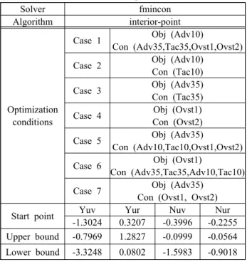
Table 3 shows an overall condition of the optimization process. The interior point method is one of the algorithms to solve linear and nonlinear convex optimization problems. It provides an optimal solution by traversing the interior of the feasible region. In this study, four linear hydrodynamic co- efficients of sway force and yaw moment are selected as input
variables and seven different objective function and constraints are provided to the optimization process. Turning manoeuvre with 10 degrees and 35 degrees of rudder angle and zigzag manoeuvre with 10 degrees of rudder angle are used for the optimization. Advance and tactical diameter of the turning ma- noeuvre, first and second overshoot angle of the zigzag ma- noeuvre are the detailed items to be compared with the ob- jective and constraint functions.
The initial variable and lower and upper bounds are also important conditions of the optimization. They limit the range of the variables of the optimization. The initial variable is the value of 'Norrbin' in Table 2. The optimization will start from the original regression value. The values of lower and upper bounds are calculated –50% and 200% of ship's original di- mensions, which affects the calculation of hydrodynamic co- efficients, respectively.
Solver fmincon
Algorithm interior-point
Optimization conditions
Case 1 Obj (Adv10)
Con (Adv35,Tac35,Ovst1,Ovst2)
Case 2 Obj (Adv10)
Con (Tac10)
Case 3 Obj (Adv35)
Con (Tac35)
Case 4 Obj (Ovst1)
Con (Ovst2)
Case 5 Obj (Adv35)
Con (Adv10,Tac10,Ovst1,Ovst2)
Case 6 Obj (Ovst1)
Con (Adv35,Tac35,Adv10,Tac10)
Case 7 Obj (Adv35)
Con (Ovst1, Ovst2)
Start point Yuv Yur Nuv Nur
-1.3024 0.3207 -0.3996 -0.2255 Upper bound -0.7969 1.2827 -0.0999 -0.0564 Lower bound -3.3248 0.0802 -1.5983 -0.9018 Table 3: Detailed conditions of optimization
where,
- Obj: Objective function
- Con: Nonlinear equality constraints - Adv :Advance from turning manoeuvre - Tac: Tactical diameter from turning manoeuvre - Ovst: Overshoot angle from zigzag manoeuvre
4. Verification of optimization results
Table 4 shows the optimization results and compares their manoeuvre characteristics with the benchmark data and initial regression data. Manoeuvring data from the turning circle test with rudder angle 10 and 35 degrees and the zigzag test with rudder angle 10 degrees were used for comparison. As shown
in the table, result of Case 1 is almost the same with the benchmark data. Results of Case 5 and Case 7 are also close to the benchmark data than others. It is supposed that at least two different manoeuvres with various rudder angle are required to get successful optimization results. However Case 6 showed that the overshoot angles of the zigzag manoeuvre are not proper for the condition of the objective function. Results of Case 1, 5 and 7 are similar with the benchmark data. Other results show re- stricted manoeuvring characteristics corresponding to their con- ditions of the objective function and constraints, respectively.
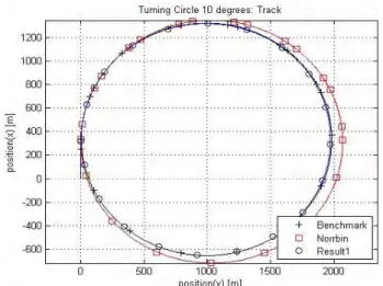
Figures 8-10 compare simulation results of the benchmark data, results using the Norrbin coefficients and the results of the optimization results of case 1. The optimized simulation is fitted to the trajectory of the benchmark data.
Figure 8: Result of optimization: Turning circle 35
Condition Coefficients Manoeuvre characteristics
Yuv Yur Nuv Nur Adv35 Tac35 Adv10 Tac10 Ovst1 Ovst2
Benchmark - -0.9000 1.2500 -0.1500 -0.2250 351.57 567.86 1072.6 1980.9 1.6342 1.7645
Norrbin - -1.3024 0.3207 -0.3996 -0.2255 330.81 501.92 1098.2 2068.6 1.5907 1.6255
Case 1
TC10 (Obj) TC35,ZZ10
(Con)
-0.8942 1.2492 -0.1501 -0.2255 351.00 566.56 1069.9 1974.0 1.6366 1.7700
Case 2 TC10 (Obj)
TC10 (Con) -0.7991 1.0247 -0.1002 -0.2116 345.23 546.91 1078.8 1976.3 1.6253 1.7466 Case 3 TC35 (Obj)
TC35 (Con) -1.8854 0.7481 -1.1338 -0.2681 351.14 566.88 1158.9 2199.7 1.4534 1.4760 Case 4 ZZ10 (Obj)
ZZ10 (Con) -1.2241 0.2339 -1.2673 -0.3756 342.41 495.66 1085.7 2004.9 1.6258 1.7566
Case 5
TC35 (Obj) TC10,ZZ10
(Con)
-0.9796 1.2446 -0.1360 -0.2263 350.99 565.35 1069.9 1973.6 1.6371 1.7727
Case 6
ZZ10 (Obj) TC35,TC10
(Con)
-3.3248 0.2153 -0.4933 -0.1993 327.57 497.01 1069.2 2003.7 1.6553 1.7124
Case 7 TC35 (Obj)
ZZ10 (Con) -0.8045 1.2433 -0.1522 -0.2247 350.74 566.19 1067.8 1968.1 1.6383 1.7732 Table 4: Optimization results
Figure 9: Result of optimization: Turning circle 10
Figure 10: Result of optimization: Zigzag 10/10
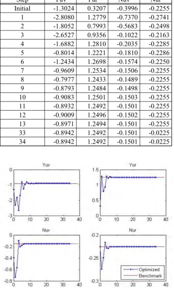
Table 5 and Figure 11 show how long the algorithm needs to find the optimal results. During 35 steps of the overall opti- mization process, actual optimization is completed near the 10th step. After that, minor corrections to find the minimum between the benchmark data and the optimized data are con- tinuing until the end of the process.
Step Yuv Yur Nuv Nur
Initial -1.3024 0.3207 -0.3996 -0.2255
1 -2.8080 1.2779 -0.7370 -0.2741
2 -1.8052 0.7993 -0.5683 -0.2498
3 -2.6527 0.9356 -0.1022 -0.2163
4 -1.6882 1.2810 -0.2035 -0.2285
5 -0.8014 1.2221 -0.1810 -0.2286
6 -1.2434 1.2698 -0.1574 -0.2250
7 -0.9609 1.2534 -0.1506 -0.2255
8 -0.7977 1.2433 -0.1489 -0.2255
9 -0.8793 1.2484 -0.1498 -0.2255
10 -0.9083 1.2501 -0.1503 -0.2255
11 -0.8932 1.2492 -0.1501 -0.2255
12 -0.9009 1.2496 -0.1502 -0.2255
13 -0.8971 1.2494 -0.1501 -0.2255
33 -0.8942 1.2492 -0.1501 -0.0225
34 -0.8942 1.2492 -0.1501 -0.0225
Table 5: Optimization histories of coefficients
Figure 11: Optimizing histories of coefficients
5. Conclusion
This paper studied an optimization process to suggest a tun- ing process for ship modelling. The turning manoeuvre with rudder angel 35 degrees and 10 degrees and zigzag manoeuvre with rudder angle 10 degrees were carried out to compare be- tween the benchmark data and the optimized data. A short brief of this study is as follows:
Firstly a double-ended ferry with two pairs of azimuth pro- pulsion units was adopted as the target vessel. Prior to the op- timization process, modelling the vessel was carried out by
MATLAB/Simulink. The mathematical model was borrowed from the model of MSCW simulator in Germany.
Secondly, an optimization algorithm and multiple optimal conditions of the objective function and nonlinear equality constraints, were provided to be verified. Turning manoeuvre and zigzag manoeuvre and their manoeuvre characteristics were used to the optimization conditions and verification.
Finally, optimized results for easy case are compared with the benchmark simulation data. The optimal conditions which apply at least two different manoeuvres with various rudder angle showed satisfactory simulation results compared to the benchmark data. There was a limit for other optimization con- ditions where the simulation result could not satisfy for all manoeuvres.
However, the target values of this study were limited to four linear hydrodynamic derivatives and even though these four values have dominant influence on the manoeuvring char- acteristics of certain vessels, there is a need for additional re- search to optimize more hydrodynamic derivatives for certain mathematical models. Also the environmental influence should be considered in the future studies.
References
[1] International Towing Tank Conference, “The manoeu- vring committee: Final report and recommendations to the 25th ITTC,” Proceedings of 25th ITTC, vol. 1, pp. 145-152, 2008.
[2] P. Oltmann, “Identification of hydrodynamic damping derivatives - A progmatic approach,” International Conference on Marine Simulation and Ship Manoeuvrability, vol. 3, Paper 3, pp. 1-9, 2003.
[3] J. Seils, Die Identifikation der hydrodynamischen Parameter eines mathematischen Modells fur die ges- teuerte Schiffsbewegung mit Verfahren der nichtli- nearen Optimierung, Ph.D Dissertation, Fakultät für Mathematik, Natur- und Technikwissenschaften, Hochschule für Seefahrt Warnemünde-Wustrow, Germany, 1990 (in German).
[4] M. A. Abkowitz, “Measurement of hydrodynamic characteristics from ship maneuvering trials by system identification,” Society of Naval Architects and Marine Engineers, vol. 88, pp. 283-318, 1980.
[5] K. Rhee and K. Kim, “A new sea trial method for es- timating hydrodynamic derivatives,” Journal of Ship and Ocean Technology, vol. 3, no. 3, pp. 25-44, 1999.
[6] X. Zhang and Z. Zou, “Identification of Abkowitz model for ship manoeuvring motion using -support
vector regression,” Journal of hydrodynamics, vol. 23, No. 3, pp. 353-360, 2011.
[7] K. T. Tran, A. Ouahsine, F. Hissel and P. Sergent,
“Identification of hydrodynamic coefficients from sea trials for ship maneuvering simulation,” Proceedings of Transport Research Arena 5th conference, 2014.
[8] Z. Zou, Ship manoeuvring and seakeeping, Shanghai, China, Shanghai Jiao Tong University, 2006.
[9] N. H. Norrbin, Theory and Observations on the Use of a Mathematical Model for Ship Manoeuvring in Deep and Confined Waters, Technical report of Swedish Steel Producers Association (SSPA), No. 68, Gothenburg, Sweden, 1971.
[10] D. Clarke, P. Gedling and G. Hine, “The application of manoeuvring criteria in hull design using linear theory,” Royal Institution of Naval Architects, Vol.
125, pp. 45-68, 1983.
[11] A. Minchev, C. Simonsen and R. Zilcken,
“Double-ended ferries: propulsive performance chal- lenges and model testing verification,” Proceedings of the second International Symposium on Marine Propulsor, Hamburg, 2011.
[12] J. Nocedal and S. J. Wright, Numerical optimization, Second edition, Springer, 2006.