Vol. 23, No. 3, pp. 258-265, May 31, 2017, ISSN 1229-3431(Print) / ISSN 2287-3341(Online) https://doi.org/10.7837/kosomes.2017.23.3.258
1
1. Introduction
The need for ship modelling technology is continuously growing with the development of marine information technology.
Ship modelling is necessary not only for conventional demands, such as early ship design stages and real-time ship simulation, but also for various forms of fast time simulation for education and training (Benedict et al., 2014). Given this rapid technological development, the importance of simple and efficient ship modelling method is still increasing.
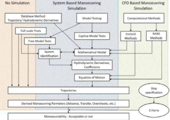
Estimating hydrodynamic coefficients for a ship model is one important stage in determining ship manoeuvrability with high accuracy. Especially for the submerged part of the hull, the forces and moments at work can be presented via hydrodynamic coefficients. The International Towing Tank Conference (ITTC) summarized different methods (Fig. 1) to estimate hydrodynamic coefficients to determine ship manoeuvrability (ITTC, 2008). Each method has individual accuracy, effort and cost characteristics, but the captive model test and Computational Fluid Dynamics (CFD) method are commonnly used at the design stage (Oltmann,
Corresponding Author : [email protected]
2003; Seils, 1990). These methods are the most reliable source of hydrodynamic coefficients, excluding full scale trials, which require relatively high cost and calculation time compared to an empirical method with system identification.
This paper applies a system identification method using sea trial data. It estimates the hydrodynamic coefficients for a ship model via a mathematical optimization algorithm. This algorithm compares results of manoeuvre simulation with benchmark data, such as sea trial data, and it provides updated, optimized target variables.
Various ideas on system identification have been studied with the progress of computational calculations. The Extended Kalman Filter (EKF) has been widely used since the beginning of the development of this method (Abkowitz, 1980; Hwang, 1980), and System Based (SB) free running tests have also been carried out with the EKF algorithm (Rhee and Kim, 1999; Zahng and Zou, 2011). Other mathematical algorithms have also been introduced with the development of computers, such as Sequential Quadratic Programming (SQP) and Broyden-Fletcher-Goldfarb-Shanno (BFGS) (Saha and Sarker, 2010; Tran et al., 2014).
Kim et al. optimized hydrodynamic coefficients with an interior point algorithm, based on simulation manoeuvre data as a
Estimation of Hydrodynamic Coefficients from Sea Trials Using a System Identification Method
Daewon Kim
*Knud Benedict
**Mathias Paschen
**** Graduate School, Faculty of Mechanical Engineering and Marine Technology, University of Rostock, Albert-Einstein-Strasse 2, 18059 Rostock, Germany
** ISSIMS Institute, Hochschule Wismar, University of Applied Sciences, Technology, Business and Design, Richard-Wagner-Strasse 31, 18119 Rostock, Germany
*** Faculty of Mechanical Engineering and Marine Technology, University of Rostock, Albert-Einstein-Strasse 2, 18059 Rostock, Germany
Abstract : This paper validates a system identification method using mathematical optimization using sea trial measurement data as a benchmark. A fast time simulation tool, SIMOPT, and a Rheinmetall Defence mathematical model have been adopted to conduct initial hydrodynamic coefficient estimation and simulate ship modelling. Calibration for the environmental effect of sea trial measurement and sensitivity analysis have been carried out to enable a simple and efficient optimization process. The optimization process consists of three steps, and each step controls different coefficients according to the corresponding manoeuvre. Optimization result of Step 1, an optimization for coefficient on x-axis, was similar compared to values applying an empirical regression formulae by Clarke and Norrbin, which is used for SIMOPT. Results of Steps 2 and 3, which are for linear coefficients and nonlinear coefficients, respectively, was differ from the calculation results of the method by Clarke and Norrbin. A comparison for ship trajectory of simulation results from the benchmark and optimization results indicated that the suggested stepwise optimization method enables a coefficient tuning in a mathematical way.
Key Words : Mathematical optimization, Ship manoeuvrability, System identification method, Hydrodynamic coefficients, Sea trial
preliminary study (Kim et al., 2016). This paper presents a second validation of the suggested optimization algorithm. The benchmark data set consists of sea trial results for the training ship Hanbada of the Korea Maritime and Ocean University.
Comparison among the benchmark data, initial condition of the optimization process and finally optimized data are also presented in this paper.
Fig. 1. Overview of manoeuvring prediction methods.
2. Modelling ship and benchmark data
2.1 Mathematical model
The 3-Degrees-of-Freedom (DOF) ship-fixed and Earth-fixed coordinate systems are applied in this study, and Fig. 2 presents the relevant concepts where the Earth-fixed-coordinate plane and the ship-fixed-coordinate plane lie on an undisturbed free surface, with the axis pointing in the direction of the original heading of the ship, while the axis and the axis point vertically downwards. The angle between the and axes is defined as the heading angle, .
Fig. 2. Coordinate system for the vessel.
where,
: Center of gravity
: Heading
: Drift angle
: Rudder angle
: Ship speed
: Yaw rate
The fast time simulation tool SIMOPT, of the ISSIMS Institute from Hochschule Wismar was used for simulation in the optimization process (Fig. 3). This tool uses almost the same ship dynamic features as the Ship Handling Simulator (SHS) systems (ANS5000) developed by Rheinmetall Defence Electronics (ISSIMS GmbH, 2013). In the mathematical model used for this tool, a ship is considered a massive and rigid body.
Forces and moment acting on the hull are described as in equation (1), according to the Newtonian law of motion (Rheinmetall Defence Electronic, 2008).
(1)
Fig. 3. Data input interface for SIMOPT.
Each value for force and moment in the model consists of multiple modules, as in Equation (2): hull, propeller, rudder and other external forces and moments. Environmental factors are considered in the following chapter.
(2)
Equation (3) shows the composition of the hydrodynamic forces and moment acting on the hull. In this model, empirical regression formulas by Norrbin and Clarke are applied to calculate initial hydrodynamic coefficients (Norrbin, 1971; Clarke et al., 1983). Each hydrodynamic coefficient can be expressed as a function of the ship’s main dimensions, as in Equation (4):
length, beam, draught and displacement of the ship. and
are non-linear components of sway force and yaw moment.
These non-linear components are dependent on the position of the ship’s turning point.
′ ′ ′ ′ ′ ′
′ ′ ′ ′ ′ ′
′ ′ ′ ′ ′ ′
(3)
′ ′ ′ ′ ′ ′
∆ (4)2.2 Benchmark data
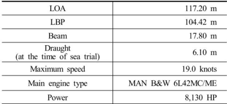
The training ship Hanbada has been adopted as a benchmark vessel for the optimization process, and the particulars of this vessel are given in Table 1.
LOA 117.20 m
LBP 104.42 m
Beam 17.80 m
Draught
(at the time of sea trial) 6.10 m
Maximum speed 19.0 knots
Main engine type MAN B&W 6L42MC/ME
Power 8,130 HP
Table 1. Particulars of T/S Hanbada
The environment is one of the biggest factors that influences manoeuvre characteristics between the towing tank model experiment and the full-scale sea trial. Controlling and calibrating environmental factors are important for obtaining accurate mathematical optimization results from the sea trial. Thus, a correction method provided by the International Maritime Organization (IMO) has been applied to calibrate track coordinates for the sea trial results. The detailed procedure is as follows (IMO, 2002).
To measure environmental influence, turning circle test results are required. The recorded data should include the ship’s track,
heading and the time elapsed with at least a 720° change of heading. In terms of the data, two half-circles can be obtained after a heading change of 180° from the beginning of the test.
Local current velocity
can be defined using two corresponding positions ′′ ′ and ′ ′ ′ , from the half-circles drawn as Equation (5):
(5)
From local velocity, estimated current velocity can be calculated, as in Equation (6):
(6)
The magnitude of current velocity can be calculated using Equation (7):
(7)The final corrected trajectories from the measured data can be obtained from Equation (8):
′
(8)
where
is the measured position vector and
′ is the corrected vector for the ship, with
′
at .
Fig. 4. Corrected trajectory (1): TC35S.
Fig. 5. Corrected trajectory (2): TC35P.
Fig. 4 and 5 show a comparison of the measured sea trial trajectory and the calibrated trajectory. The magnitude and direction of current velocity are also applicable to other manoeuvres.
3. Optimization of hydrodynamic coefficients
3.1 Mathematical optimization
Mathematical optimization is a process that minimizes or maximizes an objective function value, subject to several variable constraints (Nocedal and Wright, 2006). This can be expressed as in Equation (9):
∈
min , subject to (9)
∈
≥ ∈
where,
- is the variable to be optimized, which normally should be a vector
- is an objective function which returns a scalar and contains information for minimization or maximization - are constraints, sets of equations and inequalities that
variable must satisfy throughout the optimization process.
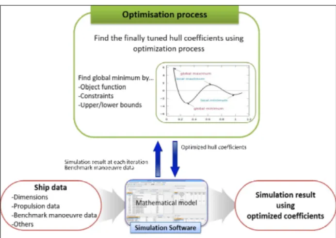
The MATLAB Optimization Toolbox calculates various kinds of optimization problems, such as constrained, unconstrained, continuous and discrete problems, using popular optimization solvers and algorithms. Fig. 6 shows the whole process of mathematical optimization for hydrodynamic coefficients.
Fig. 6. Concept flow for mathematical optimization.
Solvers require an objective function to provide a minimum or maximum value to optimize of target values. In order to improve the reliability and accuracy of the result of the optimization process, additional constraints may be required. A lower and upper bound, linear and non-linear equalities and linear and non-linear inequalities are representational constraints that may be involved in the optimization process.
3.2 Sensitivity analysis
The estimated time required for mathematical optimization is highly dependent on the number of variables to be optimized. In this study, the variables are the hydrodynamic coefficients for the ship’s hull. Thus, it is important to check the sensitivity of each hydrodynamic coefficient in terms of how strongly they contribute to a ship manoeuvre, prior to conducting the optimization process. Summarized sensitivity analysis procedures are as follows:
1) Separate coefficients into three groups according to the manoeuvre tests: straight motion, manoeuvre with a small rudder angle and manoeuvre with large rudder angle.
2) Change the specific coefficient from a value close to 0 for each sign to 10 times the original value, and conduct simulation.
3) Find the derivative of non dimensional manoeuvre characteristics with respect to the change of coefficient and divide this by the greatest value of the manoeuvre characteristics values for normalization.
4) Repeat for all coefficients.
Fig. 7 to 9 show the results of the sensitivity analysis, and Table 2 shows the list of coefficients to be optimized. The optimization process in this study consists of three phases. Step 1 optimizes two coefficients that represent the force acting on the x-axis. Step 2 takes four linear sway and yaw coefficients using a result from zigzag manoeuvre with a rudder angle of 10 degrees, which represents a manoeuvre with a small rudder angle.
Step 3 takes nonlinear coefficients using a result from turning manoeuvre with a rudder angle of 35 degrees, which represents a manoeuvre with a large rudder angle.
Fig. 7. Result of sensitivity analysis (1): straight motion.
Fig. 8. Result of sensitivity analysis (2): with small rudder angle.
Fig. 9. Result of sensitivity analysis (3): with large rudder angle.
Optimization Step Coefficients Remarks
Step 1 Xuu Xu4 Straight motion
Step 2 Yuv Yur Nuv Nur Small rudder angle Step 3 Xvr Yvr Nrr Nvv Large rudder angle Table 2. Detailed conditions for optimization
3.3 Optimization conditions
Table 3 shows the overall conditions for the optimization process. As mentioned in Subsection 3.2, a stepwise process is applied for optimization. Trajectory differences between the benchmark data and the simulation results based on optimized coefficients are selected as objective functions. The optimization results from the previous step are also applied as initial conditions for the next optimization step.
Step 1 Step 2 Step 3
Solver fmincon
Algorithm interior-point
Initial values
Xuu -0.0458 Yuv -1.5336 Xvr 1.0225 Xu4 -0.3490 Yur 0.3245 Yvr 1.7265 Nuv -0.5796 Nrr 0.1079 Nur -0.2429 Nvv 0.8633
Lower bounds
Xuu -0.4000 Yuv -15.336 Xvr 0.0001 Xu4 -3.0000 Yur 0.0001 Yvr 0.0001 Nuv -5.7960 Nrr 0.0001 Nur -0.2429 Nvv 0.0001
Upper bounds
Xuu -0.0001 Yuv -0.0001 Xvr 10.000 Xu4 -0.0001 Yur 3.2450 Yvr 17.000 Nuv -0.0001 Nrr 1.0790 Nur -0.0001 Nvv 8.6330 Objective
function
Track difference straight
motion
zigzag 10 degrees
turning circle 35 degrees
Constraints none none none
Table 3. Detailed conditions for optimization
4. Verification of optimization results
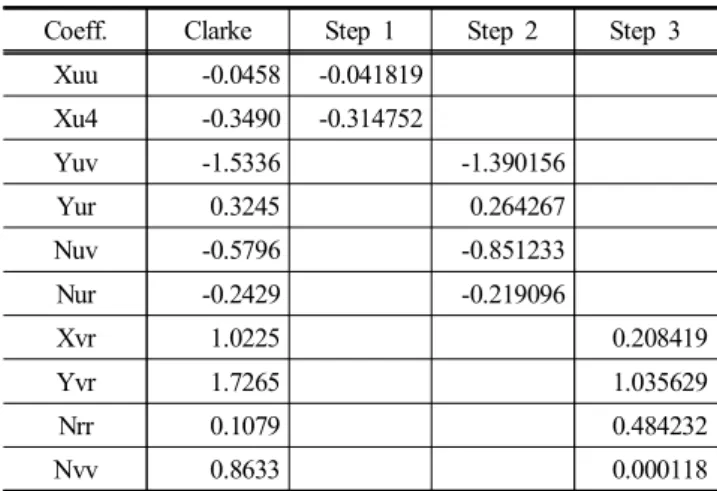
Table 4 presents the optimization results, and Table 5 compares the manoeuvre characteristics from the benchmark data, the simulation results using coefficients found via Clarke estimation and the results of all the optimization steps. The
coefficients from Step 1 are relatively similar to the Clarke estimations, compared to results from other steps. Fig. 10 shows that all of the simulation results indicate similar trajectories.
Coeff. Clarke Step 1 Step 2 Step 3
Xuu -0.0458 -0.041819
Xu4 -0.3490 -0.314752
Yuv -1.5336 -1.390156
Yur 0.3245 0.264267
Nuv -0.5796 -0.851233
Nur -0.2429 -0.219096
Xvr 1.0225 0.208419
Yvr 1.7265 1.035629
Nrr 0.1079 0.484232
Nvv 0.8633 0.000118
Table 4. Optimization results: hydrodynamic coefficients
Way/Lpp Ovst1 Ovst2 Adv35 Tac35
Benchmark 23.40 7.20 12.70 298.00 399.50
Clarke 23.01 3.10 4.70 298.16 432.11
Step 1 23.43 3.30 4.60 300.30 435.46
Step 2 23.43 9.00 17.40 225.34 281.95
Step 3 23.43 7.30 14.10 287.79 398.46
Remarks first
overshoot second
overshoot advance tactical diameter Table 5. Optimization results: manoeuvre characteristics
Fig. 10. Comparison of optimization results: straight motion.
Fig. 11 and 12 present the trajectory and heading changes for a zigzag manoeuvre, based on the optimization results from each step and compare these outcomes with the benchmark data. This shows that the simulation results from Steps 2 and 3 are close to the benchmark data, and the nonlinear coefficients optimized in Step 3 had little effect on the results of the Step 2.
Fig. 11. Comparison of optimization results: zigzag manoeuvre with a rudder angle of 10 degrees (track).
Fig. 12. comparison of optimization results: zigzag manoeuvre with a rudder angle of 10 degrees (heading).
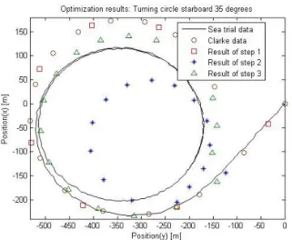
Fig. 13 shows the trajectory for a turning manoeuvre. The result of Step 2 indicated that linear coefficients have a big influence on turning manoeuvres, though this influence could be negative or positive. The results of Step 3 showed that selected nonlinear coefficients can help manage a ship’s manoeuvre characteristics, especially for manoeuvre with large rudder angle.
Fig. 13. Comparison of optimization results: turning manoeuvre with a rudder angle of 35 degrees.
5. Conclusion
This paper focused on an optimization process for hydrodynamic coefficients when modelling ships. The approach to basic mathematical optimization used here was derived from the authors’ latest research, and benchmark data was gathererd from a sea trial. A short summary of the study is as follows:
First, the training ship Hanbada was used to gather measured benchmark data. A sea trial was performed using the procedures suggested by IMO. The measured data was calibrated to correct for environmental influences on the raw values measured.
Second, basic modelling and simulation for optimization were carried out using fast time simulation tool SIMOPT, provided by the ISSIMS Institute in Germany. This tool applied a mathematical model for an ANS 5000 simulator by Rheinmetall Defence and this estimates hydrodynamic coefficients acting on the hull by empirical regression following the Clarke and Norrbin method.
Finally, the optimization process itself was composed of three steps: a straight motion, a yaw checking manoeuvre with a small rudder angle and a turning manoeuvre with a large rudder angle.
Prior to starting the optimization process, a sensitivity analysis was carried out and the coefficients to be optimized were chosen.
Each step involved different coefficients to avoid interference, and the corresponding results were satisfactory in comparison with the benchmark data.
In future studies, more optimization results based on sea trial data should be collected to identify differences between existing
empirical estimation formulas and to suggest new regression formulas.
References
[1] Abkowitz, M. A.(1980), Measurement of Hydrodynamic Characteristics from Ship Maneuvering Trials by System Identification, SNAME Transactions, Vol. 88, pp. 283-318.
[2] Benedict, K., M. Kirchhoff, M. Gluch, S. Fischer, M.
Schaub, M. Baldauf and S. Klaes(2014), Simulation Augmented Manoeuvring Design and Monitoring - A New Method for Advanced Ship Handling, The International Journal on Marine Navigation and Safety of Sea Transportation, Vol. 8, No. 1, pp. 131-141.
[3] Clarke, D., P. Gedling and G. Hine(1983), The Application of Manoeuvring Criteria in Hull Design Using Linear Theory, Transactions of the RINA, London, pp. 45-68.
[4] Hwang, W. Y.(1980), Application of System Identification to Ship Maneuvering, PhD thesis, MIT.
[5] IMO(2002), International Maritime Organization, Explanatory Notes to the Standards for Ship Manoeuvrability, MSC/Circ.
1053.
[6] ITTC(2008), The Manoeuvring Committee Final Report and Recommendations to the 25th ITTC, Proceedings of 25th ITTC, Vol. 1, pp. 145-152.
[7] Kim, D. W., M. Paschen and K. Benedict(2016), A Study on Hydrodynamic Coefficients Estimation of Modelling Ship using System Identification Method, Journal of the Korean Society of Marine Engineering, Vol. 40, No. 10, pp.
935-941.
[8] Kirchhoff, M.(2013), Simulation to Optimize Simulator Ship Models and Manoeuvres (SIMOPT), Software Manual, Innovative Ship Simulation and Maritime Systems GmbH (ISSIMS), Rostock.
[9] Nocecdal, J. and S. J. Wright(2006), Numerical Optimization - second edition, Springer.
[10] Norrbin, N. H.(1971), Theory and Observations on the Use of a Mathematical Model for Ship Manoeuvring in Deep and Confined Waters, SSPA Publication, No. 68, Gothenburg.
[11] Oltmann, P.(2003), Identification of Hydrodynamic Damping Derivatives - a Progmatic Approach, International Conference on Marine Simulation and Ship Manoeuvrability, Vol. 3, Paper 3, pp. 1-9.
[12] Rhee, K. P. and K. Kim(1999), A New Sea Trial Method for Estimating Hydrodynamic Derivatives, Journal of Ship and Ocean Technology, Vol. 3, No. 3, pp. 25-44.
[13] Rheinmetall Defence Electronic(2008), Advanced Nautical Simulator 5000 (ANS 5000) - Software Requirement Specification (SRS), Company Publication, Bremen.
[14] Saha, G. K. and A. K. Sarker(2010), Optimization of Ship Hull Parameter of Inland Vessel with Respect to Regression Based Resistance Analysis, Proceedings of The International Conference of Marine Technology 2010 (MARTEC).
[15] Seils, J.(1990), Die Identifikation der hydrodynamischen Parameter eines mathematischen Modells für die gesteuerte Schiffsbewegung mit Verfahren der nichtlinearen Optimierung, Doktorarbeit der Hochschule für Seefahrt Warnemünde-Wustrow.
[16] Tran, K. T., A. Ouahsine, F. Hissel and P. Sergent(2014), Identification of Hydrodynamic Coefficients from Sea Trials for Ship Maneuvering Simulation, Transport Research Arena 2014, Paris.
[17] Zhang, X. and Z. Zou(2011), Identification of Abkowitz Model for Ship Manoeuvring Motion using -support Vector Regression, Journal of Hydrodynamics, Vol. 23, No.
3, pp. 353-360.
Received : 2017. 05. 10.
Revised : 2017. 05. 23.
Accepted : 2017. 05. 29.