Median Filtering Detection using Latent Growth Modeling

논문 2015-52-1-8

잠재성장모델링을 이용한 미디언 필터링 검출

( Median Filtering Detection using Latent Growth Modeling )

이 강 현^**

( Kang Hyeon RHEE

)

요 약

최근에 위,변조 영상의 처리이력 복구를 위한 포렌식 툴로서 미디언 필터링 (MF: Median Filtering) 검출기가 크게 고려되 고 있다. 미디언 필터링의 분류를 위한 미디언 검출기는 적은 양의 특징 셋과 높은 검출율을 갖도록 설계되어야 한다. 본 논문 은 변조된 영상의 미디언 필터링 검출을 위한 새로운 방법을 제안한다. BMP를 미디언 윈도우 사이즈에 의하여 여러 미디언 필터링 영상으로 변환하고, 윈도우 사이즈에 따른 차분포 값을 계산하여 그 값으로 미디언 필터링 윈도우 사이즈와 같은 특징 셋을 만든다. 미디언 필터링 검출기에서, 특징 셋은 잠재성장 모델링 (LFM: Latent Growth Modeling)을 사용하는 모델 특성 으로 변환된다. 실험에서, 테스트 영상은 TP (True Positive)와 FN (False Negative) 두 분류로 판별된다. 제안된 알고리즘은 분류 효율성이 TP와 FN의 혼동에서 최소거리 평균이 0.119로서 훌륭한 성능임이 확인 되었다.

Abstract

In recent times, the median filtering (MF) detector as a forensic tool for the recovery of forgery images’ processing history has concerned broad interest. For the classification of MF image, MF detector should be designed with smaller feature set and higher detection ratio. This paper presents a novel method for the detection of MF in altered images. It is transformed from BMP to several kinds of MF image by the median window size. The difference distribution values are computed according to the window sizes and then the values construct the feature set same as the MF window size. For the MF detector, the feature set transformed to the model specification which is computed using latent growth modeling (LGM). Through experiments, the test image is classified by the discriminant into two classes: the true positive (TP) and the false negative (FN). It confirms that the proposed algorithm is to be outstanding performance when the minimum distance average is 0.119 in the confusion of TP and FN for the effectivity of classification.

Keywords :Median filter, Median filtering detector, Digital image forensics, Latent growth modeling (LGM), Structural equation modeling (SEM).

* 평생회원, 조선대학교 전자정보공과대학 전자공학과 (Chosun University, College of Electronics and Information Eng., Dept. of Electronics Eng.)

ⓒ Corresponding Author (E-mail: [email protected])

※ 본 논문은 조선대학교 2010 교비지원(322386)으로 수행되었습니다.

접수일자: 2014년11월08일, 수정일자: 2014년12월01일 게재확정: 2015년01월02일

Ⅰ. 서 론

In the image alterations, the content-preserving manipulation is using compression, filtering, averaging, rotate, mosaic editing and scaling and so on, using the forgery method.^[1～2] Median filtering is especially preferred among some forgers because it has characteristics of non-linear filtering based on

order statistics. Furthermore, median filtering may affect the effectiveness of different steganalysis techniques.^[3～8] Consequently, the median filtering (MF) detector becomes a significant forensic tool for the recovery of the processing history of a forgery image.

To detect MF in forgery images, G. Cao et al.^[6]

analyzed the probability that an image's first-order pixel difference is zero in textured regions. In this regard, Ray Liu^[9] account for the scheme which is highly accurate in unaltered or uncompressed images.

In this paper, the author focused on the discrimination of an unaltered or altered image by MF, and the classification of window size, if an image is median filtered. Also, the author attempted to reduce the number of feature set for MF detection. To create a difference distribution from window sizes which are the same as the median filtering window size 3×3 (MF3), 5×5 (MF5) and 7×7 (MF7) respectively in each MFw, w∈{3, 5, 7}, and it has different eight level anchor pixel values ai, where i∈{1, 2, … , 8}.

The proposed algorithm is formed by using structural equation modeling (SEM) to classify MFw. The SEM in this paper is formed using latent growth modeling (LGM) which assigns the statistical properties to the measurement variables as an exogenous variable in the model.

The rest of the paper is organized as follows. In Section Ⅱ, it briefly presents a theoretical background of MF operation. In Section Ⅲ, it describes the construction of the new feature set, and the method to classify the MFw by the formed SEM using LGM for the proposed algorithm. The experimental results of the proposed algorithm are shown in Section Ⅳ, the performance estimation is compared with prior arts, and followed by some discussions. Finally, the conclusion is drawn, and the future work is presented in Section Ⅴ.

Ⅱ. Theoretical Background of MF Operation

The median pixel values obtained from overlapping filter windows related to one another since overlapping windows share several pixels in common.^[5]

The median in statistic means the value in the middle of the items or literally halfway down the list of items ⎾w/2⏋.

≡







 

 

  

 i f   





 



  

 i f   

. (1)

where

By using median operation, a noise signal in audio and image can be removed due to its nonlinear nature. Also, median filtering of image is capable of smoothing and denoising a signal while preserving its edges within a content.

Let’s consider median

M×N grayscale image G

with (m,n)∈{1, 2, … , M}×{1, 2, … , N}, a 2-D median filter is defined as

   

{

}. (2)

where _{  } is the median filtered image at image coordinates (m,n). MF{·} is the median operator, and

w(m,n) is the 2-D filter window centered at the

그림 1. 미디언 필터링에 의한 위,변조 영상 Fig. 1. Forgery image produced by median filtering.

square windows as it is the most widely used form of median filtering.^[10]

In the forensics community, median filtering is considerably used. Fig. 1 shows the Lena image altered using MF{·} for a forgery by w.

Ⅲ. Proposed Algorithm of MF Detection

This paper describes the construction of a new feature set at the different window sizes around an anchor pixel which has eight different level values for consistent MF detection in digital images.

Moreover, the methods for both focusing to reduce the number of the feature set and smaller window size than existing techniques is contrived. For the proposed algorithm, a new feature set will be constructed, and SEM will be used to discriminate unaltered images, or median filtering will be formed using LGM in this Section.

And, if it is the median filtered image, which is classified the window size of a median filtering.

Thus, for the construction of the feature set, the proposed algorithm in this paper is composed of four functional routines as follows:

1) Smaller to reduce the number of feature sets, 2) Smaller to window size of MF detector,

3) Forming the model specification of SEM, that discriminates an unaltered image and median filtered,

4) Classify the window size, if median filtered.

3.1 New Feature Set of MF Detector

In a grayscale image, the pixel value is an integer in the set

P={0, 1, … , 255}. In Fig. 2, the image

그림 2. A 의 고정 픽셀

Fig. 2. Anchor pixel values in A .

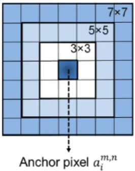
그림 3. 고정 픽셀 주변의 윈도우 사이즈 Fig. 3. Window size around an anchor pixel.

numerals) then the anchor pixel value (numerals in acircle) is set to the center value of each level. Eight anchor pixel value ais are in set

A={15, 47, 79, 111,

Let three window types w (3×3, 5×5 and 7×7) denote the window sizes around each anchor pixel coordinate _^{  } in Fig. 3, where w={3,5,7} and (m,n) is a coordinate.

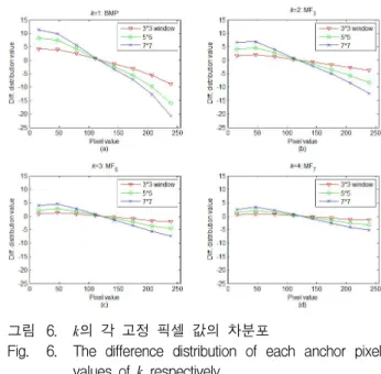
The difference distribution values _^ are computed according to w size around _^{  } by Eq. 3.

_^



   ⌊⌋

⌊⌋

   ⌊⌋



⌊⌋

_^{  } _{ }

,

(3)

where (x,y) and (m,n) (1, … , M)×(1 , … , N), and

M×N is the size of an image. As a result. 

_ 



  



_^

.

(4)

Thus, the feature set of the image has three values constructed from three widow sizes. Each window size is the same as MFw respectively.

3.2 Forming SEM for MF Detector

First of all, to form SEM to discriminate an unaltered image or median filtered, a measurement

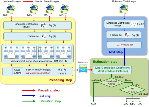
그림 5. 미디어 필터링 검출의 제안된 알고리즘 Fig. 5. The proposed algorithm for MF detection.

그림 4. 미디언 필터 영상 분류를 위한 비조건 LGM의 측정 모델

Fig. 4. The measurement model of an unconditional LGM for the classification of the median filtered image.

model should be presented with an unconditional LGM.

For the MF detector, Fig. 4 shows the measurement model measurement variable if it is median filtered, where ICEPT (Initial score), SLOPE (Rate of change),

e (Error) and X (Measurement variable by median

F

and X7 for repeat measurement analysis. Thus, the

measurement variable Xw is formed as

__{  }



  

·_{ · }



  

 

, (5)

where w={3,5,7}.

3.3 Proposed algorithm

A flow diagram of the proposed algorithm for the MF detector is shown in Fig. 5. The preceding step is to compute the model specifications of SEM Sk

(refer in Fig. 7) for the unaltered and median filtered images already known, where (k=1: unaltered image BMP, k=2: MF3, k=3: MF5 and k=4: MF7).

In the test step block, when some image is not known at all, _^ and Fw of a test image is computed and then _ (test image's Fw) into the estimation step block, which is called _.

Lastly, in the estimation step block, the Euclidean distance and the correlation coefficient between Sk

and _ are computed by (6) and (7) considering the maximum correlation coefficient and the minimum Euclidean distance for the discrimination of the test image T. True positive (TP) means that the discrimination is accomplished and false negative (FN) means that it failed respectively.

If T is median filtered, according to k, median filtering window size is classified by (8).

TP = max(Corrcoef(Sk,_)) ∪ min(Euclidean(k,_))

{if k =1 both T= BMP

if 2≥ ^k both T=MF ^w , (6)

FN = max(Corrcoef(Sk,_)) ∩ min(Euclidean(k,_))

{if k =1 both T= BMP

if 2≥ ^k both T=MF ^w . (7)

From Eq. (5)-(7) and the coefficients of ICEPT and SLOPE in Fig. 4, a new discriminant is derived as Eq. (8) and (9) for classifying k and w of MF images.

__{  }



  

·_{ · }



  

 

(8)

  











_

 _i f    i f   

_ i f   

. (9)

Ⅳ. Experimental Results

4.1. Developing the model specification for the MF detector.

The effectiveness of the proposed MF detection algorithm is extensively evaluated using the BOW2 original image database of 10,000^[11], and its median filtered 30,000 (MF3, MF5 and MF7 artificial

그림 6. k의 각 고정 픽셀 값의 차분포

Fig. 6. The difference distribution of each anchor pixel values of k respectively.

tampered images) produced with w (3, 5 and 7), for a total of 40,000 images.

The experiment is progressed as follows:

[Step 1] Each k (in Section 3.3) has 10,000 images and the difference distribution _^ of all images is computed by (6) at each ai in

A (Fig. 2). Around

[Step 2] For the reliability of the feature set, the Z-score of each image at k=1 (BMP: univariate normality) is computed from the average pixel value of an image. If the Z-score is |1.96| @ Significance level 0.05, it can not be used in the sample image. The number of available test images is 8,815 excepted 1,185 outlier images due to normality.

[Step 3] Fw

(each w of k) is respectively inputted as

in Fig. 4. The paths

with 0, 1 and 2 under an assumed positive linear. This step is executed on Amos 21 (IBM® SPSS®).

Table 1 illustrates the test of goodness-of-fit in [Step 3]. Through the results of sample images, the goodness of fit is satisfaction.

Model BMP MF3 MF5 MF7

Hair et al.

AVE

ICEPT 0.58 0.45 0.39 0.40 SLOPE 0.20 0.19 0.17 0.17

표 1. 적합도의 테스트 결과

Table 1. The results of the test of goodness-of-fit.

BMP Sem.AStructure (Model specifications) ("BMP_w3=(1.00)ICEPT+(.00)SLOPE+(1)e1") ("BMP_w5=(1.00)ICEPT+(1.00)SLOPE+(1)e2") ("BMP_w7=(1.00)ICEPT+(2.00)SLOPE+(1)e3") ("SLOPE <--> ICEPT (146.72)")

("ICEPT (20.90, 784.38)") ("SLOPE (14.62, 341.76)") ("e1 (0, -223.73)") ("e2 (0, 199.10)") ("e3 (0, -441.20)")

MF3 Sem.AStructure (Model specifications) ("MF3_w3=(1.00)ICEPT+(.00)SLOPE+(1)e1") ("MF3_w5=(1.00)ICEPT+(1.00)SLOPE+(1)e2") ("MF3_w7=(1.00)ICEPT+(2.00)SLOPE+(1)e3") ("SLOPE <--> ICEPT (59.71)")

("ICEPT (15.89, 105.28)") ("SLOPE (16.28, 99.17)") ("e1 (0, -17.48)") ("e2 (0, 18.45)") ("e3 (0, -35.88)")

MF5 Sem.AStructure (Model specifications) ("MF5_w3=(1.00)ICEPT+(.00)SLOPE+(1)e1") ("MF5_w5=(1.00)ICEPT+(1.00)SLOPE+(1)e2") ("MF5_w7=(1.00)ICEPT+(2.00)SLOPE+(1)e3") ("SLOPE <--> ICEPT (27.09)")

("ICEPT (10.60, 38.50)") ("SLOPE (11.35, 41.13)") ("e1 (0, -1.63)") ("e2 (0, 1.95)") ("e3 (0, 5.46)")

MF7 Sem.AStructure (Model specifications) ("MF7_w3=(1.00)ICEPT+(.00)SLOPE+(1)e1") ("MF7_w5=(1.00)ICEPT+(1.00)SLOPE+(1)e2") ("MF7_w7=(1.00)ICEPT+(2.00)SLOPE+(1)e3") ("SLOPE <--> ICEPT (15.43)")

("ICEPT (7.79, 25.87)") ("SLOPE (8.34, 24.12)") ("e1 (0, -1.79)") ("e2 (0, 2.00)") ("e3 (0, 3.53)")

그림 7. Amos에서 미디언 필터링 검출의 구조방정식 모델링의 모델특성

Fig. 7. The model specifications of SEM for MF detection on Amos.

where Hair et al. AVE (convergent validity): OK 0.5 higher (BMP is the initial basis of the several tampered images) on Amos.

The proposed MF detection algorithm is executed on the measurement model of an unconditional LGM for the model specifications, which are like the path coefficient, the variance and covariance of the latent variable, and the structural equation for SEM. These model specifications on Amos are presented in Fig. 7.

LGM of BMP, MF3, MF5 and MF7 is drawn, and the structural equation with its coefficients and the error values of the measurement variables are presented respectively.

Until here, it is the preceding step of the proposed algorithm in Fig. 5.

4.2. Estimation of MF detector

In the estimation step block in Fig. 5, by Eq. (6) and (7), BMP and MF images are discriminated with

S

T

k.

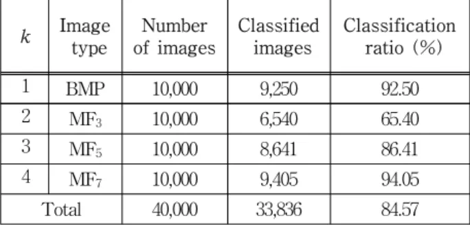
In order to relieve the proposed algorithm, the k’s combinational table is suggested in Table 3, and the results of Table 2 is estimated for the performance with the confusion matrix (TP and FN), ROC (Receiver Operating Characteristic curve) and Pe (Minimum average decision). If so, what types of image are classified well? Which could be proven with a lower value by Pe as

k Image type

Number of images

Classified images

Classification ratio (%)

1 BMP 10,000 9,250 92.50

2 MF3 10,000 6,540 65.40

3 MF5 10,000 8,641 86.41

4 MF7 10,000 9,405 94.05

Total 40,000 33,836 84.57

표 2. 미디언 필터에서 윈도우 사이즈 분류

Table 2. Classification of window size, if median filtered.

Label BMP MF3 MF5 MF7

ROC Number Pe

of TP

Number of FN

Sensitivity (TP rate)

1-Specificity (FP rate)

A − − − − 0 2,324 0.768 1 0.384

B − − − ◯ 3 738 0.693 1 0.347

C − − ◯ − 1 664 0.627 0.999 0.314

D − − ◯ ◯ 32 242 0.603 0.998 0.302

E − ◯ − − 0 462 0.557 0.996 0.280

F − ◯ − ◯ 7 212 0.536 0.996 0.270

G − ◯ ◯ − 2 173 0.519 0.996 0.261

H − ◯ ◯ ◯ 705 61 0.512 0.999 0.258

I ◯ − − − 254 2,814 0.231 0.925 0.153

J ◯ − − ◯ 653 863 0.145 0.900 0.123

K ◯ − ◯ − 164 681 0.077 0.834 0.121

L ◯ − ◯ ◯ 2,353 217 0.055 0.818 0.119

M ◯ ◯ − − 86 311 0.024 0.583 0.221

N ◯ ◯ − ◯ 356 98 0.014 0.574 0.220

O ◯ ◯ ◯ − 88 95 0.005 0.538 0.233

P ◯ ◯ ◯ ◯ 5,296 45 0 0.530 0.235

Total 10,000 10,000 1 1

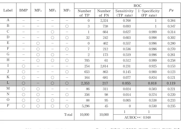
AUROC**: 0.948 표 3. k의 조합테이블에 포함된 혼동 매트릭스, ROC 그리고 Pe.

AUROC는 0.948로서, 0.9 이상은 ‘Excellent’로 평가

Table 3. The k’s combinational table involves the confusion matrix, ROC and Pe.

** AUROC (Area Under ROC curve): 0.948, and Estimation: 0.9 higher (Excellent).

그림 8. 제안된 미디언 필터링 검출기의 ROC 커브와 Pe

Fig. 8. ROC curve and Pe for the proposed MF detector.

Schemes Feature set AUROC

The proposed MF detector

Difference distribution

to feature set. 0.948

[6] Post-sharpened 0.923

[7] Post-sharpened 0.525

[8] Post-sharpened 0.706

표 4. 기존의 AUROC와 제안된 미디언 필터링 검출 기의 비교

Table 4. AUROC compared between prior arts and the proposed MF detector.

  min 

_{ }  _



, (10)

where PFP is FP rate, and PTP is TP rate respectively.

According to k, TP and FN, and its ROC curve are shown in Table 3. As a result, at the lowest

Pe=0.119 (in Label L) the outstanding performance is

carried out.

The ROC curve and the Pe are drawn in Fig. 8 and the compared results between the proposed and prior arts are presented in Table 4.

V. Conclusion

In the classification of the MF image, the typical works have tried to reduce the number of the feature sets and the window size for extracting a feature vector, and yet they increase the MF detection ratio.

In the classification of the MF image, the typical works have tried to reduce the number of the feature sets and the window size for extracting a feature vector, and yet they increase the MF detection ratio.

In this paper, the MF detector for the construction of the feature set is proposed, which has smaller window sizes, same as the median filtering sizes.

Through a series of experiments, the discriminant is formed with coefficients of the model specification of SEM; using an unconditional LGM. The coefficients are computed using a growth structure of LGM, which is like a window size (3→5→7).

Additionally, the experimental results show that the proposed MF detector can more reliably discriminates between unaltered and median filtering than the existing median filtering forensic techniques.

Moreover, its window size is also classified if median filtered is to be outstanding performance when Pe=

0.119 in the confusion of TP and FN for the effectivity of classification.

REFERENCES

[1] Kang Hyeon RHEE, “Image Forensic Decision Algorithm using Edge Energy Information of Forgery Image,” Journal of the Institute of Electronics and Information Engineers, Vol. 51, No. 3, pp. 75-81, Mar. 2014.

[2] Il Yong CHUNG and Kang Hyeon RHEE,

“Traitor Traceability of Colluded Multimedia Fingerprinting code Using Hamming Distance on

XOR Collusion Attack,” Journal of the Institute of Electronics and Information Engineers, Vol.

50, No. 7, pp. 175-180, July. 2013.

[3] M. Kirchner and J. Fridrich, “On detection of median filtering in digital images,” in Proc.

SPIE, Electron. Imaging, Media Forensics and Security II, vol. 7541, pp. 1-12, 2010.

[4] A. D. Ker and R. Böhme, “Revisiting weighted stego-image stegoanalysis,” in

Proc. SPIE, Electron. Imaging: Security, Forensics, Steganography and Watermarking of Multimedia Contents X, Vol. 6819, p. 5, 2008.

[5] Xiangui Kang, Matthew C. Stamm, Anjie Peng, and K. J. Ray Liu, “Robust Median Filtering Using an Autoregressive Model,” IEEE Trans.

on Information Forensics and Security, Vol. 8,

[6] G. Cao, Y. Zhao, R. Ni, L. Yu, and H. Tian,

“Forensic detection of median filtering in digital images,” in Multimedia and Expo (ICME), 2010, Jul. 2010, pp. 89–94. 2010.

[7] H. Yuan, “Blind forensics of median filtering in digital images,” IEEE Trans. Inf. Forensics

Security, vol. 6, no. 4, pp. 1335-1345, Dec.2 011.

[8] Matthias Kirchner and Rainer Bȫhme, “Tamper hiding: Defeating image forensics.,” in Infor.

Hiding ’07, Jun. 2007, pp. 326–341, 2007.

[9]

Stamm, M.C., Min Wu, Liu, K.J.R.,

Access IEEE, pp. 167-200, 2013.

[10] C. Chen, J. Ni, R. Huang, and J. Huang, “Blind median filtering detection using statistics in difference domain,” in Proc. of Infor. Hiding ’12, May 2012.

[11] http://bows2.ec-lille.fr/ (Aug. 2014)

저 자 소 개 이 강 현(평생회원)

대한전자공학회논문지, 51권3호 (2014. 03) 참조.