1. Introduction
High crime rates in urban neighborhood have been interests in many criminology studies since the Shaw and McKay’s work (1942). Related to crime occurrences, urban areas are characterized to have greater crime intensity as the bigger the places are (Brantingham and Brantingham 1984).
Though there are many factors deriving greater crime occurrences in urban areas, the distinguished
demographic features are size, density, and heterogeneity (Bottoms and Wiles 1995, 1997, Clinard 1978, Wikstrom 1991). Size of population is one of the most remarkable features of a city.
Huge population size in limited urban space results in high population density, consequently causing frequent stranger-to-stranger contacts among residents. These contacts among strangers form indifferent and superficial relations among residents. In addition, the population heterogeneity
* This study is supported by a College of Education of Korea University Grant
An Analysis of Urban Residential Crimes using Eigenvector Spatial Filtering*
Youngho Kim
Abstract : The spatial distribution of crime incidences in urban neighborhoods is a reflection of their socio-economic environment and spatial inter-relations. Spatial interactions between offenders and victims lead to spatial autocorrelation of the crime incidences. The spatial autocorrelation among the incidences biases the interpretation of the ecological model in OLS framework. This research investigates residential crimes using residential burglaries and robberies occurred in the city of Columbus, Ohio, for 2000. In particular, the spatial distribution of incidence rates of residential crimes are accounted in OLS framework using eigenvectors, which reflect spatial dependence in crime patterns.
Result presents that handling spatial autocorrelation enhanced model estimation, and both economic deprivation and crime opportunity are turned out significant in estimating residential crime rates.
Keywords : Environmental Criminology, Spatial Autocorrelation, Spatial Filtering, Eigenvector
in urban areas increase frictions among the residents (Wirth 1938) and enforce the anonymous and superficial relations because of their various social and economic back ground.
The anonymous and superficial relations in urban neighborhoods naturally lead to more crime opportunities showing higher crime rates (Herbert 1982, Krivo and Peterson 1996). Based on these urban characteristics, many criminology studies have analyzed relationship between crime rates and their socio-demographic features in urban neighborhoods. As a result, in explaining high crime rates, several neighborhood features have been found significant such as poverty, racial heterogeneity, family structure, and level of social control (Land, et al. 1990, Peterson, et al. 2000, Sampson and Lauritsen 1994). However, as Morenoff et al. notes (2001), the relationship between neighborhood features and the crime rates are still not clear how the relations generate various and inconsistent analysis results among studies.
This study assumes that neglecting spatial effects of crime data has been one of the main obstacles in crime analysis. Many statistical crime analyses link human socio-economic factors to the spatial distribution of crimes. However, many studies do not handle spatial effects of crime appropriately, causing problems in statistical crime analysis models (Mencken and Barnett 1999, Messner, et al.
1999). Among spatial effects, spatial autocorrelation has been noted in many studies. Described as similarity (and systematic dissimilarity) in values of nearby locations (Cliff and Ord 1981), spatial autocorrelation is commonly formed by both direct and indirect interactions between victims and offenders (Craglia, et al. 2001, Messner, et al. 1999,
Sampson and Morenoff 2004). Failing to control spatial autocorrelation may generate biased or(and) inefficient analysis results in Ordinary Least Square (OLS) framework making the analysis result misleading (Fomby, et al. 1984, Fox 1997, Kim 2008, McMillen 2003, Tiefelsdorf 2000) Though many studies test the existence of spatial autocorrelation, the efforts to handle spatial autocorrelation was quite recently emerged in environmental criminology. For instance, to account for spatial autocorrelation, Lyon (2007) and Kane (2005) used Spatially Lagged component, Jones-Webb et al (2008A, 2008B) applied Conditional Autoregressive component, and Andresen (2006) applied Simultaneous Autoregressive components. Handling spatial autocorrelation would be meaningful. However, appropriate control of spatial autocorrelation using optimally constructed spatial components based on underlying spatial process of data would be far more desirable in spatial crime analysis.
This study aims to control spatial autocorrelation in residential crime analysis by appropriately accounting for spatial patterns of data using a spatial filtering method by Griffith. The spatial filtering method uses eigenvectors generated from spatial weight matrix. In particular, set of selected eigenvectors capture spatial autocorrelation component in the OLS residuals. As a result, efficient and unbiased parameter estimation becomes possible. This study, by using spatial filtering method, has relative advantages compared to others. First, compared to spatial regression models, the use of the spatial filtering method enables optimal control of spatial autocorrelation regardless underlying spatial process. Meticulously selected eigenvectors controls not only positive
spatial autocorrelation but also negative spatial autocorrelation when required. Second, in contrast to maximum likelihood estimation (MLE), the spatial filtering method does not need distribution information of applied data. In addition, computational load is negligible compared to MLE.
Third optimal capturing spatial autocorrelation using eigenvectors enables to visualize underlying spatial process of data by decomposing data into trend, signal, and noise (Haining 1990).
Composed of residential burglary and robberies, the residential crime analyzed in this study has several advantages for crime analysis. First, the data itself provide exact location information.
Compared to other crime types such as street robbery or highway theft, residential crimes provide accurate address information of crime location generated from victims’ address. Further, security issues and corresponding privacy protection programs keep both crime offenders’
and victims’ location information concealed.
Second, residential crimes have advantages in analyzing urban neighborhood problems. As noted by Shaw and McKay (1942), crime incidents have systematic relationships with socio-economic features of a neighborhood. Naturally, urban residential crime can be constructively used to understand urban problems in both ecological and demographical perspectives.
This study is organized as follows. The section on data description presents data generation, transformation process by empirical Bayes estimation, variable selection, and its background.
The methodology presents general framework of spatial filtering methods using eigenvectors, and two applied models are introduced. The result section presents eigenvector selection process, the
regression results of the two models, and their interpretation. In particular, the results present map visualization of spatial autocorrelation pattern captured from residential crime data. The conclusion summarizes the major findings in this study.
2. Data description and variable generation
The original crime data were collected and reported by the Columbus police department.
Organized by Uniform Crime Reporting (UCR) codes of 119 different types of crime, the data are collection of all crime occurred within the areas of Columbus police precincts from Jan. 1st to Dec.
31st in 2000. The data contain specific address information, census tract numbers (based upon 1990 census tract configuration), and exact dates of occurrences. According to the crime classifications of UCR program, the residential crimes are composed of robberies and burglaries targeted at residential units. Under UCR definitions, robbery is defined as “The taking or attempting to take anything of value from the care, custody or control of a person or persons by force or threat of force or violence and/or putting the victim in fear”, and burglary is defined as “The unlawful entry (forceful or not) of a structure to commit a felony or theft”
(Federal Bureau of Investigation 2000). Table 1 shows the lists of applied residential crimes, their UCR codes, and descriptions defined by Federal Bureau of Investigation.
The data were organized by the coverage area of 19 Columbus police precincts. Since the data was
created and managed by Columbus police department, the use of the police precincts is justifiable. As a result, the study area is not completely overlaid by the city boundary missing several incorporated areas such as Bexley, Whitehall, Worthington, and Upper Arlington.
These incorporated areas maintain their own police departments and manage crime cases using their own police forces. Defining study area, Census tract were considered in addition to the police precincts. As a result, overall 9672 residential crime occurrences, composed of both residential burglary (9192 cases) and residential robbery (480 cases), were used for the analysis.
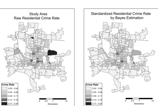
Residential crime rates were calculated by dividing crime occurrences with the number of household for each Census tract. Figure 1 present residential crime rates within study area. Standardized by the number of household, the spatial pattern of the residential crime rates shows clustering of high crime rates around central city area, implying positive spatial autocorrelation.
When the probability of an observed count in an area is significantly different from the expected value, it would be appropriate to apply smoothing technique to stabilize variance in the raw data (Langford 1994). In the crime data used in this
study, some areas have unrealistically high crime rates calculated by their small population size.
Given that a residential crime rate is calculated by dividing residential crime counts with the number of household, the corresponding rate value would have large variance when the number of household is small. In Figure 1, the dark colored area of high crime rates is characterized by very small population size and corresponding high crime rates because of international airport and large school campus. As a result, small population size boosted crime rates in the areas, in spite of small number of residential crime occurrences, making crime rates unrealistically high.
This problem was handled by applying empirical Bayes estimation (Bayes smoothing). The Empirical Bayes estimation can be described as a parameter estimation based on the degree of confidence in both the observed parameter and prior knowledge of the parameter (Bailey and Gatrell 1995). When a true and unknown rate is θi, and an observed rate is ri=yi/ni, empirical Bayes estimation parameter, θˆi, is defined as follow,
θˆi=wiri+(1-wi)γi (1) Table 1. Residential crimes and their UCR codes
Crime Types UCR Codes Descriptions
Robbery 3150 Robbery using Gun Targeted at Residence 3250 Robbery using Knife Targeted at Residence 3350 Robbery using Others Targeted at Residence 3450 Robbery using Hands Targeted at Residence Burglary 5111 Forcible Entry to Residence at Day time
5112 Forcible Entry to Residence at Night
Where wi=
And, the best parameter estimate of θiis assumed to have prior probability distribution with mean γi
and variance фi. For computational convenience γi
and фiare replaced by global estimation of mean γ˜`= and variance ф˜`= - ·yi is an observed crime count, and ni is an the size of population at risk with mean value n°. wi is shrinkage estimate reflecting the level of the confidence in the observed value ri. wiis decided by size of population, ni. For instance, when population size of an area is large, large ni value makes wivalue close to 1, leading Bayes estimated value θˆiclose to observed value ri, and vice versa.
Figure 2 present the crime rate patterns adjusted by
empirical Bayes estimation. The two areas of exceptionally high crime rate areas are adjusted by the population size.
Census tract 2000 SF1 and SF3 were applied to present neighborhood socio-economic status.
Initial variables were selected based on Land et al(1990)’s work which reviews previous literature about significant urban neighborhood socio- demographic features. Overall, as shown in Table 2, the independent variables reflect social theories that explain the relationship between crimes and urban neighborhoods. The use of income and residential stability variables is justified by social disorganization theory1 (Bursik 1988, Shaw and McKay 1942).
γ˜ n°
∑ni(ri-γ˜)2
∑ni
∑yi
∑ni
фi
фi+γi/ni
Figure 1. Study Area & Raw Crime Rate Figure 2. Adjusted Crime Rate by Empirical Bayes Estimation
3. Methodology
Regarding eigenvector generation and selection, it should be noted that major framework of the methodology in this study is heavily dependent on Tiefelsdorf and Griffith (2007). This study applied eigenvector filtering methods for two spatial process: Simultaneous Autoregressive (SAR) process and Spatial Lag (Lag) process. The main reason of applying two different spatial processes is that these two processes present different statistical features and may generate different results. Defined as y=Xβ+ρVy-ρVXβ+η, SAR process presents that unbiased and efficient regression parameters are estimated when spatial autocorrelation component, ρVy-ρVXβ, is appropriately accounted (Fomby, et al. 1984, Tiefelsdorf and Griffith 2007). In the equation, V is spatial link matrix, ρspatial autocorrelation parameter, and ηis white noise2. However, when the spatial autocorrelation component is not accounted in SAR process, parameter estimation is inefficient but unbiased (see for detail, Fox 1997 p.
126-129). The unbiased parameter estimation, even under spatial autocorrelation in residuals, is explained by zero correlation between spatial autocorrelation component and independent variable: Corr(X, ρVy-ρVXβ)=0. However, under Lag process y=Xβ+ρVy+η, the situation is a little different. The correlation between independent variable and spatial autocorrelation component, Corr(X, ρVy)≠0, makes the parameter estimation biased when spatial autocorrelation component is not appropriately accounted.
Eigenvectors have unique features that a set of eigenvectors generated are intrinsically orthogonal to each other having zero correlation. In addition, generated from spatial link matrix, V, eigenvectors present hypothetical spatial patterns of possible spatial autocorrelation under spatial link matrix topology (Griffith 1996, 2003). When properly generated, eigenvectors may represent spatial properties in both SAR process and Lag process and be used as spatial proxy variables (Tiefelsdorf and Griffith 2007). Two projection matrices and corresponding two eigenvectors can be considered. A projection matrix with matrix of Table 2. Variables and their description
Variable Category Source (areal units) Variable Generation
Residential crime rate Police crime data, Residential crime cases SF1 (Block) / No. of residences Number of residential units Crime opportunity SF1 (Block) Number of residential units Median family income Economic status SF3 (Tract) Median family income Divorce rate Family structure SF3 (Block group) Divorced population
/ Population 5 years and more Rate of living in a same Residential SF3 (Block group) Population living in a house
house 5 years and more stability 5 years and more
/ Population 5 years and more
independent variables X is formed as follow. Also, corresponding eigenvector is,
M(X)=I-X(XTX)-1XT (projection matrix) (2)
{e1, ..., en}SAR=evec[M(X)VM(X)]
(corresponding eigenvectors) (3)
Given ESARis a eigenvector matrix whose vectors are drawn from {e1, ..., en}SAR, ESAR is intrinsically orthogonal to independent variables X. Seeing that spatial component in SAR process is not correlated to independent variables, eigenvector matrix ESAR
can be used as proxy variables to capture spatial component in SAR process: ESARγ≈ρVy-ρVXβ.
Similarly, a projection matrix with a unit vector 1 and corresponding eigenvector is,
M(1)=I-1(1T1)-11T (projection matrix) (4) {e1, ..., en}Lag=evec[M(1)VM(1)]
(corresponding eigenvectors) (5)
Similar to SAR process, eigenvector matrix ELag
from {e1, ..., en}Lagcan be used as proxy to account for Lag process because The eigenvector matrix ELag is not necessarily orthogonal to independent variables X : ELagγ≈ρVy.
Appropriate spatial autocorrelation filtering in OLS models requires suitable set of eigenvectors.
Two types of eigenvector selection algorithm can be considered: (1) maximizing r-square method by Griffith (2003) and (2) minimizing Moran’s I method by Tifelsdorff (2007). The two methods, as the name implies, are characterized by using r- square values and Moran’s I values as a reference in selecting eigenvectors. The r-square method
uses straightforward stepwise regression procedures. Specifically, eigenvectors are selected by their statistical significant in order. For instance, an eigenvector with high absolute t-values in OLS framework are selected in advance. Seeing that the stepwise procedure is implemented in almost statistical software, the method is relatively easier to be applied in eigenvector selection procedure compared to the Moran’s I method.
The Moran’s I method measures changes of spatial autocorrelation εlevel in residuals as an eigenvector eiis applied. Setting OLS residuals with spatial autocorrelation as a dependent variable and eigenvector as an independent variable, OLS model would be as follow with ηias residuals in the model,
ε=γ0+γ1e1+ηi (when one eigenvector is applied) ε=γ0+γ1e1+γ2e2+η2
(when two eigenvectors are applied) (6) ε=γ0+γ1e1+γ2e2+...+γnen+ηn
(when n eigenvectors are applied)
Given that the goal is removing spatial autocorrelation in ε, it means that the iteration procedure of adding eigenvectors can be finished only when Moran’s I value of ηnshould be close to zero after n iterations. In the process, eigenvectors were selected which maximizing the different between Moran’s I values of ηiand ηn+1.
In spite of technical differences in their application, both methods do not show significant differences in their application results (Tiefelsdorf and Griffith 2007). This study applied the Moran’s I method. Although r-square method is relatively more convenient than Moran’s I method for application, the Moran’s I method is more
parsimonious using smaller number of eigenvectors. In addition, using many eigenvectors may increase unnecessary multicollinearity in the model because of increased correlation among independent variables and eigenvectors.
4. Result
1) Eigenvector selection
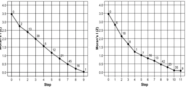
Minimizing Moran’s I method was applied for eigenvector selection. Figure 3 present changes in spatial autocorrelation level of residual ηi in equation (6) as selected eigenvectors are added one by one. The steps in X-axis present the iteration process adding eigenvectors and Y-axis present corresponding Moran’s I values of ηi for each step. As more eigenvectors are applied, corresponding Moran’s I values of ηi is declined.
The selection of eigenvectors was stopped just one
step before the Moran’s I value of ηi became negative. Since this study used only eigenvectors with positive eigenvalues which portray positive spatial autocorrelation patterns, selected eigenvectors have positive eigenvalues.
Consequently, if excessive eigenvectors are added in the filtering process, corresponding Moran’s I value of ηican become negative, forming negative spatial autocorrelation unnecessarily.
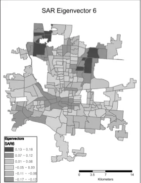
The number of eigenvectors used in each model indirectly presents the efficacy in handling spatial autocorrelation. In Figure 3, Lag process requires smaller number of eigenvectors (9) compared to the number of eigenvectors in SAR process (11) in handling spatial autocorrelation. The higher efficiency in Lag process implies that the spatial pattern in OLS residuals follows spatial Lag process rather than SAR process. Figure 4 presents the spatial patterns of the first four eigenvectors applied in SAR process for example; Eigenvector 6, 18, 8 and 1 respectively. As the map pattern
Figure 3. Changes in Moran’s I as a result of spatial filtering process (Lag process left, SAR process right)
Figure 4. Map patterns of selected SAR Eigenvectors
present similar values nearby areas, the selected (thus applied) eigenvectors present strong positive spatial autocorrelation and filters positive spatial autocorrelation in the model.
2) Regression results
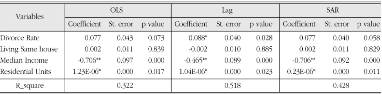
Table 3 present regression results of 3 models: 1) standard OLS, 2) OLS with Lag eigenvector filtering, and 3) OLS with SAR eigenvector filtering.
As noted in methodology chapter, eigenvectors, ESAR, generated from the projection matrix M(X)=I- X(XTX)-1XT are intrinsically orthogonal to independent variables. As a result, this orthogonal features between eigenvectors and independent variables results in same coefficient values for standard OLS model and SAR model. However, their standard errors and p_values are different.
Lag filtering model results, in contrast, show minor level of correlation between eigenvector ELag and independent variables. Naturally both coefficients and p_values are different from standard OLS model.
Overall, results follow general understanding and theories in criminology literature. Although there are notable deviations in p_values among models, signs of significant variables are consistent.
However, divorce rate, which represent family structure in neighborhood, appears significant only in Lag model with p_value 0.028. Compared to standard OLS model (p_value 0.073) and SAR model (p_value 0.058), handling spatial autocorrelation in Lag model makes significant changes in the analysis. The difference in SAR and Lag result, though minor, comes from the correlation between eigenvectors and independent variables. The result indicates that family structure is notable factors related to residential crimes even though it is not always statistically significant.
Other than family structure, criminal opportunity (the number of Residential unit) and economic status (Median Income) are significant factors to residential crime rates.
Economic status is negatively related (OLS: - 0.706, Lag: -0.465, SAR: -0.706) to residential crimes. This result indicates neighborhood with small median income has more frequent residential crimes. As shown in the literature about urban crimes (for example, Ackerman 1998, Bailey 1984, Parker and Reckdenwald 2008), economic deprivation becomes a motivator for criminal behaviors. Consequently, routine activity theory3 (Cohen and Felson 1979, Rice and Smith 2002, Smith, et al. 2000) is confirmed assuming that
Table 3 Regression result
Variables OLS ` Lag ` SAR `
Coefficient St. error p value Coefficient St. error p value Coefficient St. error p value
Divorce Rate 0.077 0.043 0.073 0.088* 0.040 0.028 0.077 0.040 0.058
Living Same house 0.002 0.011 0.839 -0.002 0.010 0.885 0.002 0.011 0.829 Median Income `-0.706** 0.097 0.000 -0.465** 0.089 0.000 -0.706** 0.092 0.000 Residential Units 1.23E-06* 0.000 0.017 1.04E-06* 0.000 0.023 0.23E-06* 0.000 0.011
R_square 0.322 0.518 0.428
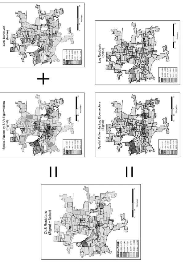
Figure 5. Map decomposition of Spatial autocorrelation components
+ = =
impoverished individuals become potential crime offenders (Bursik 1988). Crime opportunity, presented by the number of residential units, shows positive relationship to residential crimes.
Although crime opportunity varies depending on target qualities, space, time, and the offender’s preferences, this result indicates that the number of available targets is a significant factor in residential crimes. In addition, very small coefficient value of the residential unit variable is explained by the contrast between the number of residential units and crime rates. While average number of residential units per census tract is 1429, the average residential crime rate is 0.035. In spite of statistical significance, this implies that unrealistically huge increase in the number of residential units can make changes in residential crime rates. The residential stability, which is used as a proxy for social network (Coleman 1988, 1990) and social guard, does not show significant influence on residential crimes.
3) Decomposition of spatial component
Capability of capturing spatial component from residuals and mapping it is an advantage of using eigenvector spatial filtering. As Haining (1990 p.
259) noted, spatial process can be decomposed into trend, signal, and noise. Spatially autocorrelated residual εin equation (6) contains both signal and noise. Plugging in spatial filtering eigenvectors, SAR model and Lag model is decomposed as follow in this study,
y=Xβ+ρVy-ρVXβ+η Xβ+ESARγ+η(SAR model) (7) Xβ=Trend; ESARγ= signal; η= noise
y=Xβ+ρVy+η Xβ+ELagγ+η (Lag model) (8) Xβ=Trend; ELagγ= signal; η=noise
Figure 4 presents visualization of signal and noise using a map. OLS residuals present spatial patterns of combined signal and noise. From the OLS residuals, spatial autocorrelation component (signal) is captured and presented by ESARγin SAR model and ELagγin Lag model. The map patterns of ESARγand ELagγshow local clusters of similar values, which caused positive spatial autocorrelation.
5. Conclusion
This study analyzed residential crime rates using eigenvector spatial filtering methods. In data management, Bayesian smoothing was applied and adjusted unrealistically large (or small) residential crime rate values. In spatial filtering process, both Lag and SAR process were utilized to approximate underlying spatial process in OLS residuals.
Although both processes captured spatial autocorrelation component in residuals, Lag process appeared more efficient seeing the smaller number of applied eigenvectors compared to SAR process.
The results showed that economic factor (median income) was dominant in explaining residential crime rates. It implied that economic deprivation caused residential crimes by increasing motivations for criminal behavior. Although crime opportunity, approximated by the number of residential units in this study, was statistically
significant, very small coefficient value, however, made the effect of the crime opportunity on residential crime rate negligible. Family structure variable (divorce rate) was significant only in Lag model as a result of drastic decrease in p_value, compared to the same variable in standard OLS model. The map decomposition enabled to visualize spatial patterns of trend and noise.
As proxy variables, representing spatial autocorrelation components, eigenvectors can be applied to various spatial processes. Given that spatial autocorrelation is formed through various spatial processes such as diffusion, exchange and transfer, interaction, dispersal or spread (see Haining 1990 p. 24-26), eigenvectors can be utilized as proxies representing these processes.
Regarding criminology, eigenvectors can approximate and capture, for instance, migration or daily travel patterns of population. Though the eigenvectors have only filtering spatial autocorrelation in this study, future studies are expected to model underlying spatial process additionally. This study hopes to simulate further studies using eigenvectors in the field of quantitative spatial data analysis.
Note
1 The theory proposes that poverty is a factor that attracts and motivates people to engage in criminal behaviors. Additionally, the theory indicates that residential instability increases population heterogeneity, weakening social networks in a neighborhood.
2 White noise follows identical and independent normal distribution.
3 In routine activity theory, crime occurs in the place where an offender happens to be, as a result of his/her daily life-choices. Thus the offender’s daily life patterns would influence the location of offending behavior.
Reference
Ackerman, W. V., 1998, “Socioeconomic correlates of increasing crime rates in smaller communities,”
Professional Geographer 50, pp.372-387.
Andresen, M. A., 2006, “A spatial analysis of crime in Vancouver, British Columbia: a synthesis of social disorganization and routine activity theory,”
Canadian Geographer-Geographe Canadien 50, pp.487-502.
Bailey, T. C. and Gatrell, A. C., 1995, Interactive Spatial Data Analysis, Essex, England: Longman.
Bailey, W. C., 1984, “Poverty, Inequality, and City Homicide Rates: Some not so Unexpected Findings,,” Criminology 22, pp.531-550.
Bottoms, A. E. and Wiles, P., 1995, Crime and Insecurity in the City, in C. Fijnaut and Goethals J. (eds.), Changes in society, crime, and criminal justice in Europe: a challenge for criminological education and research: Kluwer Law International.
Bottoms, A. E. and Wiles, P., 1997, Environmental Criminology, in M. Maguire, Morgan R. and Reiner R. (eds.), The Oxford Handbook of Criminology:
Oxford.
Brantingham, P. J. and Brantingham, P. L., 1984, Patterns in crime, New York: Macmillan.
Bursik, R., 1988, “Social disorganization and theories of crime and delinquency: problems and prospects,”
Criminology 26, pp.519-551.
Cliff, A. D. and Ord, J. K., 1981, Spatial Process: Models and applications, London: Pion Limited.
Clinard, M. B., 1978, Cities with little crime : the case of Switzerland, New York: Cambridge University Press.
Cohen, L. E. and Felson, M., 1979, “Social change and crime rate trends: A routine activity approach,”
American Sociological Review 44, pp.588-608.
Coleman, J. S., 1988, “Social Capital in the Creation of Human Capital,” American Journal of Sociology 94, pp.95-120.
Coleman, J. S., 1990, Foundations of social theory, Cambridge: Harvard University Press.
Craglia, M., Haining, R. and Signoretta, P., 2001,
“Modelling high-intensity crime areas in english cities,” Urban Studies 38, pp.1921-1941.
Federal Bureau of Investigation, 2000, Crime in the United States, Washington, DC.: FBI.
Fomby, T. B., Hill, R. C. and Johnson, S. R., 1984, Advanced Econometric Methods, New York:
Springer-Verlag.
Fox, J., 1997, Applied regression analysis, linear models, and related models, Thousand Oaks, California:
Sage.
Griffith, D., 1996, “Spatial Autocorrelation and Eigenfunctions of the Geographic Weights Matrix Accompanying Geo-referenced Data,” The Canadian Geographer 40, pp.351-367.
Griffith, D., 2003, Spatial Autocorrelation and Spatial Filtering, New York: Springer.
Haining, R., 1990, Spatial data analysis in the social and environmental sciences, New York, NY: Cambridge University Press.
Herbert, D., 1982, The Geography of Urban Crime, New York: Longman.
Jones-Webb, R., Mckee, P., Wall, M., Pham, L., Erickson, D. and Wagenaar, A., 2008, “Alcohol and malt liquor availability and promotion and homicide in inner cities,” Substance Use & Misuse 43, pp.159-177.
Jones-Webb, R. and Wall, M., 2008, “Neighborhood racial/ethnic concentration, social disadvantage, and homicide risk: An ecological analysis of 10 US cities,” Journal of Urban Health-Bulletin of the New York Academy of Medicine 85, pp.662-676.
Kane, R. J., 2005, “Compromised police legitimacy as a
predictor of violent crime in structurally disadvantaged communities,” Criminology 43, pp.469-498.
Kim, Y., 2008, “The effects of spatial autocorrelation in spatial data analysis,” The Geographical Journal of Korea 42, pp.343-361.
Krivo, L. J. and Peterson, R. D., 1996, “Extremely disadvantaged neighborhoods and urban crime,”
Social Forces 75, pp.619-650.
Land, K. C., McCall, P. L. and Cohen, L. E., 1990,
“Structural Covariates of Homicide Rates: Are There Any Invariances Across Time and Social Space?,”
American Journal of Sociology 95, pp.922-963.
Langford, I. H., 1994, “Using Empirical Bayes Estimates in the Geographical Analysis of Disease Risk,” Area 26, pp.142-149.
Lyons, C. J., 2007, “Community (dis)organization and racially motivated crime,” American Journal of Sociology 113, pp.815-863.
McMillen, D. P., 2003, “Spatial Autocorrelation or Model Misspecification?,” International Regional Science Review 26, pp.208-217.
Mencken, F. C. and Barnett, C., 1999, “Murder, Nonnegligent Manslaughter, and Spatial Autocorrelation in Mid-South Counties,” Journal of Quantitative Criminology 15, pp.407-22.
Messner, S. F., Anselin, L., Baller, R. D., Hawkins, D. F., Deane, G. and Tolnay, S. E., 1999, “The spatial patterning of county homicide rates: An application of exploratory spatial data analysis,” Journal of Quantitative Criminology 15, pp.423-50.
Morenoff, J. D., Sampson, R. J. and Raudenbush, S. W., 2001, “Neighborhood Inequality, Collective Efficacy, and the Spatial Dynamics of Urban Violence,”
Criminology 39, pp.517-559.
Parker, K. F. and Reckdenwald, A., 2008, “Concentrated disadvantage, traditional male role models, and African-American juvenile violence,” Criminology 46, pp.711-735.
Peterson, R. D., Krivo, L. J. and Harris, M. A., 2000,
“Disadvantage and neighborhood Violent Crime: Do Local Institutions Matter?,” Journal of Research in Crime and Delinquency 37, pp.31-63.
Rice, K. and Smith, W., 2002, “Socioecological models of automotive theft: Integrating routine activity and social disorganization approaches,” The Journal of Research in Crime and Delinquency 39, pp.304-336.
Sampson, R. J. and Lauritsen, J. L., 1994, Violent Victimazation and Offending: Idividual, Situational, and community level risk factors., in A. J. Reiss and Roth J. A. (eds.), Understanding and Preventing Violence, Washington, D.C.: National Academy Press.
Sampson, R. J. and Morenoff, J. D., 2004, Spatial (Dis)Advantage and Homicide in Chicago Neighborhoods, in M. F. Goodchild and Janelle D.
G. (eds.), Spatially Integrated Social Science, New York: Oxford University Press Inc.
Shaw, C. R. and McKay, H. D., 1942, Juvenile delinquency and urban areas, a study of rates of delinquents in relation to differential characteristics of local communities in American cities, Chicago, Ill:
The University of Chicago Press.
Smith, W. R., Frazee, S. G. and Davison, E. L., 2000,
“Furthering the integration of routine activity and social disorganization theories: small units of analysis and the study of street robbery as a
diffusion process,” Criminology 38, pp.489-523.
Tiefelsdorf, M., 2000, Modelling spatial processes: the identification and analysis of spatial relationships in regression residuals by means of Moran’s I, Berlin:
Springer-Verlag.
Tiefelsdorf, M. and Griffith, D. A., 2007, “Semiparametric filtering of spatial auto correlation: the eigenvector approach,” Environment and Planning A 39, pp.1193-1221.
Wikstrom, P.-O. H., 1991, Urban Crime, Criminals, and Victims: the Swedish experience in an Anglo- American comparative perspective, New York:
Springer-Verlag.
Wirth, L., 1938, “Urbanism as a Way of Life,” American Journal of Sociology 44, pp.1-24.
교신: 김영호, 서울시 성북구 안암동, 고려대학교 사범대학 지리교육과, Tel: 02-3290-2368, Fax: 02-3290-2360, E- mail: [email protected]
Correspondence: Youngho Kim, Dept. of Geography education, Korea University, Seungbuk-Gu Seoul, Korea. Tel: +82-2-3290-2368, Fax: +82-2-3290-2360, E-mail: [email protected]
최초투고일 2009년 5월 26일 최종접수일 2009년 6월 15일
아이겐벡터 공간필터링을 이용한 도시주거범죄의 분석
김영호*
요약`: 도시에서 범죄는 해당 지역 인구의 사회경제적 특징과 공간적 상호관계를 반영한다. 범죄의 피의자와 피해자 사이의 상호작용 은 범죄패턴의 공간적 자기상관으로 나타난다. 이러한 범죄의 공간자기상관은 일반적인 최소자승모델에서 편향된 추정치를 제공하여 잘못된 해석으로 이어질 수 있다. 본 연구는 도시주거범죄로서 2000년에 오하이오주 콜럼버스에서 발생한 주거 강도와 절도를 분석 하였다. 특히 주거 범죄율의 공간적 분포패턴은 공간자기상관을 반영하는 아이겐벡터(Eigenvector)를 이용하여 최소자승모델로 분석 하였다. 아이겐 벡터를 이용한 공간자기상관의 필터링은 기존의 모델에서는 잔차에 남아있던 공간자기상관 요소를 설명하기 때문에, 더 효율적인 추정을 가능하게 하였다. 경제적 궁핍과 범죄의 기회가 주거범죄율을 추정하는데 통계적으로 유의미한 요인이었다.
주요어: 범죄분석, 공간자기상관, 공간필터링, 아이겐벡터 한국경제지리학회지 제12권 제2호 2009(179~194)
* 본 연구는 고려대학교 사범대학 특별연구비에 의하여 수행되었음