Journal of the Korean Society of Marine Engineering, Vol. 39, No. 5, pp. 554~562, 2015 ISSN 2234-7925 (Print)
J. Korean Soc. of Marine Engineering (JKOSME) ISSN 2234-8352 (Online)
http://dx.doi.org/10.5916/jkosme.2015.39.5.554 Original Paper
This is an Open Access article distributed under the terms of the Creative Commons Attribution Non-Commercial License (http://creativecommons.org/licenses/by-nc/3.0), which permits unrestricted non-commercial use, distribution, and reproduction in any medium, provided the original work is properly cited.
Design and Control of a Firefight Cannon Manipulator Applying Sliding Mode Control
Mai The Vu 1 ㆍ Hyeung-Sik Choi † ㆍ Hyeon-Seung Kang 2 ㆍ Jae-Hyeon Bae 3 ㆍ Moon-G. Joo4 ㆍ Yeong-do Joo5 (Received January 26, 2015; Revised February 12, 2015; Accepted April 9, 2015)
Abstract: This paper describes an analysis of an architecture and control system of a firefighting cannon manipulator (FCM) composed of two joint axes and one water-shooting actuator. Because the orienting FCM motion is disturbed by the reaction force from water shooting, the water shooting force has been modeled for robust control. The dynamics model of the manipulator has been set up including the external force of water-shooting reaction on the manipulator. A PD Controller and Sliding Mode Controller have been designed and their performance been tested through simulation to track a desired trajectory under the disturbance of a water- shooting reaction. The simulation shows that the performance of the Sliding Mode Controller is better than that of the PD controller.
Keywords: Firefight cannon manipulator, Controller, Kinematics, Dynamics, Simulation.
1. Introduction
In recent years, industrial robots have been evaluated for various purposes, including personal care, hazardous material treatment, fire disaster prevention, and others. Unlike industrial robots fixed at a workstation, these robots can conduct surveillance and reconnaissance by moving around the indoor and outdoor environments. This study performed a variety of tasks, including the pick-and-place task [1]. Moreover, a study of the manipulator for locomotion [2], and a study of the light weight manipulator made of carbon fiber reinforced plastic was conducted [3]. One of the best nonlinear robust controllers that can be used in uncertain nonlinear systems is the sliding mode controller (SMC), but pure SMC results in chattering in a noisy environment. This effect can be eliminated by optimizing the sliding surface slope. One study investigated a novel methodology for designing a SMC using a new heuristic search, so called "colonial competitive algorithm " to tune the sliding surface slope and the switching gain of the discontinuous part in the SMC structure [4] and another study illustrated two different control techniques for achieving finite-time convergence and continuous control [5]. These robots comprise
the locomotion part and robotic arm used in different operations.
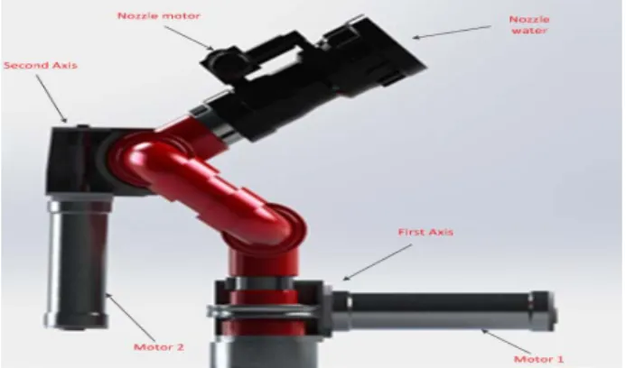
The FCM (Firefight cannon manipulator) is characterized mainly by its light weight and low degree of freedom (namely 2DOF) because it moves with a manipulator attached to the locomotion device. The features of the FMC system are shown in Figure 1.
Figure 1: Overall view of the developed FCM
The equations of motion of the manipulator have been established and analyzed by including the external force of the water impacts on a system. The performance of the SMC compensating the water impacts have been simulated by
† Corresponding Author (ORCID: http://orcid.org/0000-0002-4060-8163): Division of Mechanical and Energy System Engineering, Korea Maritime and Ocean University, E-mail: [email protected], Tel: 051-410-4969
1 Department of Mechanical Engineering, KMOU, E-mail: [email protected], Tel:051-410-4969 2 Department of Mechanical Engineering, KMOU, E-mail: [email protected], Tel:051-410-4969 3 Department of Mechanical Engineering, KMOU, E-mail: [email protected], Tel:051-410-4969
4 Department of Information and Communications Eng., Pukyong National University, Email: [email protected], Tel:051-629-6238 5 SMEC CO., Ltd, Email: [email protected], Tel: 053-524-5211
Matlab/Simulink and compared with the one of the classical PD controller.
To control the system, the PD controller and SMC have been designed to follow the desired trajectory. Simulations have been conducted to verify the availability of generated trajectories and the performance of the designed controller.
2. Architecture of FCM 2.1 Mechanical structure
The FCM is designed to perform the tasks of fire extinguishing and is composed of an elbow, swivel and nozzle.
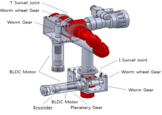
The system includes two motors (motors 1 and 2), which are used for the pan and tilt motion and the motor control nozzle are used for fog-stream. Each motor is composed of a reduction gear, DC motor and encoder. One important point in the FCM is that the gears applied are worm gears. They are used to prevent backward rotation from the reaction of water shooting.
The structures of the manipulator are composed as follows:
The manipulator joints are composed of two degrees of freedom with yawing motion of the first axis and pitching motion of the second axis, as shown in Figure 1 and 2. The first joint actuator is designed to move around in a range between 0° and 360°.
The second joint actuator is in a range from -10° to 185°.
The weights of the two links are 7.55 kg and 4.06 kg each.
The total weight of the manipulator system is approximately 11.61 kg. The manipulator has been developed to cope with a maximum load capacity of 123 kg.
Figure 2: Joints of the FCM
Table 1 lists the specification of the measured and calculated FCM and Table 2 and 3 present the parameters of motors and inertial constants.
Table 1: Parameters of the firefight cannon manipulator
Link 1 2
Length of Link, (mm) 282.81 275.56 Length of mass center (mm) 141.4 137.78
Mass, (kg) 7.55 4.06
Motion R (Yaw) R (Pitch)
Limit of angles (degrees) 0 ~360 10 ~185
Table 2: Parameters of the motors
No. Axis Motor Gear
ratio
Worm wheel 1 1st axis 272763 EC-
max30, 60 (W), 24 (V)
23:1 50:1
1 2nd axis 272768 EC- max30, 40 (W),
24 (V)
23:1 50:1
Table 3: Inertial Constants (kgm2)
Link Mass
Mi
(kg)
Inertial moment kgm2
Ixx I yy Izz
1 7.55 0.050 0.045 0.045 0
2 4.06 0.026 0.015 0.015 0
2.2 Control system
A control system has been developed to control the FCM, and the entire control system consists of a main controller, and joint motor controller, as shown in Figure 3. The main controller based on an ARM processor plays the role of editing the control algorithm, sending the order of the operation signals to the motor controller for the robot joint actuators through RS232 communication. The main controller sends continuous motion signals to motor controllers of the joint actuators according to a trajectory planning. For the joint motion controller, a STM32F207 microprocessor is applied. The controller is built in a modular control board capable of controlling two motors and has been designed to generate the Pulse Width Modulation (PWM) signal and the direction signal for the motor and to send them from the main controller to the motor driver. The motor driver has been developed to supply the power, which is proportionally amplified with the duty ratio to the joint actuating motors according to the PWM signal and the direction signal for the joint motor. Figure 4 shows a picture of water-shooting of FCM during according to control input.
Mai The Vu ㆍ Hyeung-Sik Choi ㆍ Hyeon-Seung Kang ㆍ Jae-Hyeon Bae ㆍ Moon-gap Joo ㆍ Yeong-do Joo
A proportional-derivative and feed-forward control algorithm is planned to apply to the joint controller of the developed system.
Figure 3: The developed control system
Figure 4: The water-shooting of the FCM
3. Kinematic Analysis of FCM 3.1 Forward Kinematics analysis
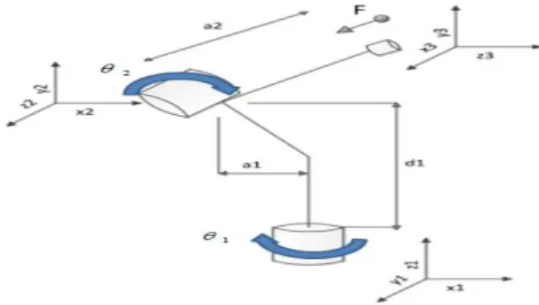
An analysis of the kinematics of FCM was performed on the joint actuator links based on a two-axis of FCM. This is because the one-axis of the manipulator is fixed on the ground surface, as the reference axis. The coordinates have been set up using the D-H (Denavit - Hartenberg) convention, as shown in Figure 5, and Tables 4 lists the corresponding joint link parameters of , , , and Each joint link is expressed as a homogeneous transformation matrix, Ai, by multiplying the two transformation matrices. The matrix of end - effector are obtained:
1 0
0 0
2 / ) ( 0
2 / ) (
2 / ) (
2 2 2 2 1 2
2
2 1 2 2 1 2 1 1 1 12 1 2
12 2 12 2 1 1 1 2 1 12
2 s c d as ls
c s l c s a s a c s s c
c l c a c a s s c c A
Table 4: Denavit - Hartenberg
Link (mm) (mm)
1 100 90 282.81
2 275.56 0 0
Figure 5: D-H coordinates of 2-axis manipulator
3.2 Inverse Kinematics analysis
Kinematic analysis was performed on joint actuator links based on a 2-axis manipulator. Since the 1-axis of manipulator was fixed on the ground surface, it was established as a reference axis. Coordinates were set up using the D-H (Denavit- Hartenberg) convention as shown in Figure 5, and then corresponding joint link parameters of ai, αi, di, and θi (where ai
is called the length, αi is called the twist, di is called the offset, and θi is called the angle, respectively) were obtained. The following Equation (1) is derived after matrix transformation through consecutive multiplication. The following Equation (1) is derived after matrix transformation through consecutive multiplication.
1 1 1
2 2 2 2
1 2
2 2
21
c s s c s
m n a a
a m n
(1)
2 2 2 2
sin m , cos n
m n m n
The following Equation (2) is obtained from Equation (1).
2 2 2 2
1 1 2
1 2 2
1
sin 2
m n a a
a m n
(2)
Similarly, the following equations are obtained.
1 1 1
2 1
2
sin sin 2 n a a
(3)
4. Dynamics Analysis of FCM
The Euler-Lagrange method is used repetitively to perform the dynamics analysis of the two-link of FCM. The dynamic equation expressing the linear and rotational motion for each
link of the manipulator is induced one after another.
The dynamic equation begins with the initial condition,
0 0 ac,0 ae,0 0 0 0T
, and the related equations are then obtained by consecutively increasing the i value from 1 to n.
4.1 Modeling of water-shooting pump
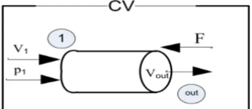
In this study, a disturbance of the system is expressed as an external force. For a control volume (CV), the second link of a system where the water move out is enclosed. The only mass flow across the CV is water moving to the right. Figure 6 shows the CV of second link.
Figure 6: Control volume of the second link The force balance is:
x out out
F F m
(4) where, mout is the mass flow, out is maximum velocity,
respectively. And the mass flow moutis given by Equation (5):
2
out out out D4
m A (5)
With Aout , and D are section area, water density and diameter of end-effector, respectively.
The final equation of water reaction force of FCM system is:
2 2
4 out
F D (6)
For the FCM system to work, it needs a water pump that can deliver a large volume of water at high pressure through a hose- like tube. This water pump will change the velocity of the water when it moves out.
In this study, maximum velocity vout14 /m s of water has been chosen to demonstrate the robustness of SMC controller.
The diameter of the shooting nozzle is D7cm and the water
density in this case is 1000(kg m/ 3) . Therefore, the maximum disturbance force is 754.3(N).
4.2 Dynamics of 2 DOF FCM In the following sections, the 2 DOF FMC dynamic equations of motion can be concisely expressed concisely as:
( ) ( , ) ( ) TE
M q q C q q q G q J F , (7)
where, q: 2x1 is position vector, : 2x1 is vector of torques, )
(q
M : 2x2 is inertia matrix of the manipulator, C( qq,): 2x2 is vector of Centrifugal and Coriolis terms,G(q): 2x1 is vector of gravity terms,JTEis Jacobian matrix and F is external forces, respectively.
Matrix M and C are symmetric 2x2 matrices:
11 12
21 22
m m
M q m m
11 12
21 22
, c c
C q q
c c
The inertia matrix is given by Equation (8),:
2 1
( ) i i i i
T T
T i T R i R
i
M q J m J J I J
, (8)where mi i, 1,2 is the mass of link each,
Ti
J and ,
Ri
J represent the Jacobian of linear velocity an angular velocity of link each, respectively.
While the Centrifugal and Coriolis matrix ( , )C q q is given by Equation (9):
( ) 1 ( )
( , ) ( ) ( )
2
T
n n
M q M q
C q q I q q I
q q
(9)
Matrix G is given by Equation (10):
i( )
i
g q q
(10)
where, Π is the potential energy of the manipulator, which is just the sum of those of the two links. For each link, the
Mai The Vu ㆍ Hyeung-Sik Choi ㆍ Hyeon-Seung Kang ㆍ Jae-Hyeon Bae ㆍ Moon-gap Joo ㆍ Yeong-do Joo
potential energy is just its mass multiplied by the gravitational acceleration and the height of its center of mass.
By starting with the end conditions of fn10, n10. The torques i of each joint are calculated consecutively. The detailed expression of Equation (8), (9), (10), and the torques
i are described in Appendix.
5. Controller Design and Computer Simulation of FCM
In this paper, the input signals used for the simulation are
1 0.1sin( )t
(rad) and 20.1cos( )t (rad). Both the PD controller and SMC have been designed and their performance been tested through simulations to track a desired trajectory under a disturbance due to a water reaction and without a disturbance. The simulation shows that the performance of the SMC is better than that of the PD controller.
5.1 Design PD Controllers and Computer Simulation The SMC and PD controller have been designed to track the desired trajectories of a vehicle and joints. A PD control algorithm is applied to control the position each link of system.
The PD control laws for each link are described in Equation (11).
p d
K e K e
(11) where , , Kpi and Kdi denote a proportional and derivative gain, respectively. The gains used for the PD controller are Kp = 90000, Kd = 600, respectively.
Figure 7 represents a block diagram of the PD controller with a disturbance.
Figure 7: Block diagram of PD controller with a disturbance
In the first simulation, the PD controller is applied to the system. The trajectory of the end-effector is assigned to move from the initial position to the target position with a constant
velocity for 10 seconds. Figure 8, 9, 10 and 11 present the simulation results. Figure 8 and 9 are the simulation results of manipulator without a disturbance. Figure 10 and 11 show the simulation results under a disturbance. The simulation shows that the measured trajectory is tracking the desired trajectory with good performance. Figure 9 and 11 show that the errors of two joints are quite small (i.e., without disturbance, the error of the first a second joint is 0° and approximately 7 10 3°. On the other hand, under the disturbance of a water reaction, the error of first joint varies from 0.01° to 0.01° and second joint is varied from 0.005° to 0.014°).
Under a disturbance, the input torques are larger than that without a disturbance (without disturbance, the input torques of the first and second link are approximately 11Nm and 0.3Nm, respectively, and under disturbance, the input torques of the first and second link are approximately 20Nm and 18Nm, respectively), as shown in Figure 9 and 11.
Figure 8: Joint angles (PD control without a disturbance)
Figure 9: Joint torques and position errors of the joints (PD control without a disturbance)
Figure 10: Joint angles (PD control with a disturbance)
Figure 11: Joint torques and position errors of joints (PD control with a disturbance)
5.2 Design of the SMC Controllers and Computer Simulation
The sliding mode method is based on the idea of keeping the scalar quantity, s, which is a weighted sum of the position error , the velocity error , and (not required) the acceleration error , at zero as reported elsewhere [6].
Here, the expression of s is chosen as expressed in Equation (12):
λ (12) where λ > 0 is the weight parameter.
Therefore, the task of the controller is to take s to zero. When s approaches zero, the position error (and velocity error, also) also approaches zero too. Therefore, and thus, trajectory tracking is performed. Once s is zero, to keep it at this value, the
derivative of s is expected to be zero. From Equation (12), the expression of s can be deduced easily as follows:
d d
s q q q q (13)
Substituting the expression of deduced from Equation (7) into Equation (13):
1 ,
( )
TE d d
s J F C q q q G q q q q
M q
(14)
So, if derivative of the scalar quantity = 0, we have:
( ) d ( ) ( d) ( ) ( , ) TE
M q q M q q q G q C q q q J F
(15)
In addition, the actual control law, which can be robust to uncertainties, is the function chosen as follows:
Ksat s
(16)
where, sat(.) is the saturating function, ㅣsat(.)ㅣ 1, ϕ > 0 is the boundary layer thickness, K is the design parameter chosen so that ㅣ ㅣ 0, with η is a strictly positive constant.
The parameters, ϕ, λ and K used for the SMC controller are ϕ
=1, 800; 800 and 500; 400 , respectively. To verify the good performance of the designed SMC, the trajectories were have been created for links and the simulation of trajectory tracking was has been carried out. Figure 12 presents the block diagram of SMC with a disturbance.
Figure 12: A block diagram of the SMC with a disturbance
In the second simulation, the SMC was applied to the system.
The trajectory of the end-effector was assigned to move from the initial position to the target position with a constant velocity
Mai The Vu ㆍ Hyeung-Sik Choi ㆍ Hyeon-Seung Kang ㆍ Jae-Hyeon Bae ㆍ Moon-gap Joo ㆍ Yeong-do Joo
for 10 seconds. Figure 13 - 16 present the simulation results.
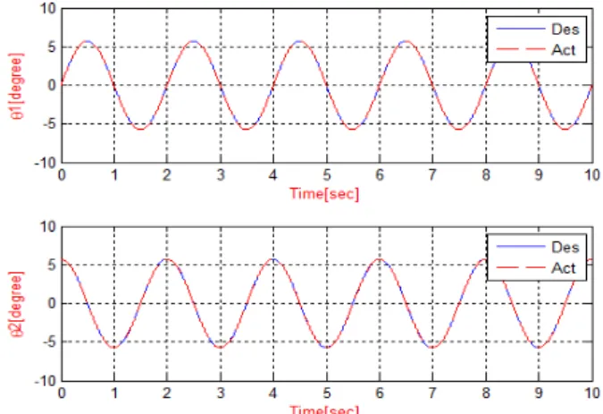
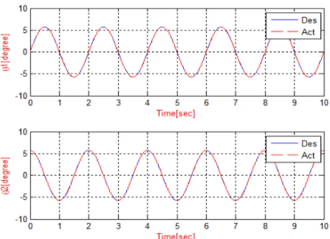
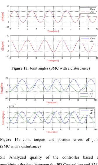
Figure 13 and 14 show simulation results of the manipulator without a disturbance. Figure 15 and 16 present the simulation results under disturbance. The simulation result shows that the measured trajectory is tracking the desired trajectory with good performance. Each joint angle is still controlled well with a disturbance. The simulation results show the validity of the SMC algorithms. Figure 14 and 16 show that the errors of the two joints are very small (i.e., without a disturbance, the error of the first and second joint is 0° and from 0.25 10 5 degrees to 0.25 10 5 degree. On the other hand, under a disturbance of the water reaction, the error of first joint varies from 2.2 10 3 degrees to 2.2 10 3 degrees and that of the second joint varies from 1.87 10 3 degree to 1.87 10 3 degree).
Under a disturbance, the input torques are larger than that without a disturbance case (without a disturbance, the input torques of the first and second link are approximately 11Nm and 0.3Nm, respectively, and under a disturbance, the input torques of the first and second link are approximately 20Nm and 18Nm, respectively), as shown in Figure 14 and 16.
Figure 13: Joint angles (SMC without a disturbance)
Figure 14: Joint torques and position errors of joints (SMC without a disturbance)
Figure 15: Joint angles (SMC with a disturbance)
Figure 16: Joint torques and position errors of joints (SMC with a disturbance)
5.3 Analyzed quality of the controller based on combining the data between the PD Controllers and SMC
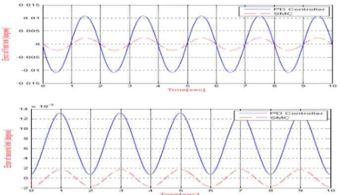
The performance of the PD Controller and SMC have been compared. Figure 17 and 18 show the simulation results of the PD Controller and SMC Controller for both cases without a disturbance and under the presence of a disturbance. According to the results, the SMC shows good trajectory tracking along the target joint angle.
Figure 17: Position errors of the joints (PD control and SMC without a disturbance)
Without a disturbance, the errors of the joints are very small, as shown in Figure 17. Under a disturbance, the simulation results show that the position errors are larger than the case without, as shown in Figure 18. Based on the results of comparing the performance of the SMC and PD controllers, the superior performance of the SMC in reducing the position errors is confirmed.
Figure 18: Position errors of the joints (PD control and SMC with a disturbance)
6. Conclusions
In this paper, a firefighting cannon manipulator (FCM) has been developed for extinguishing fires. The architecture of the developed mechanical system composed of two joint axes and one water-shooting actuator and control system for exact water shooting for fire has been described.
For the control joint of a FCM, the dynamics model of FCM composed of two joint axes and one water-shooting actuator has been set up including the external force of the water-shooting reaction on the FCM. Because the FCM motion is affected by the reaction force from water shooting, the water shooting force has been modeled.
To control the FCM accurately along the desired trajectory under an external force of a water-shooting reaction, a robust controller has been designed using the SMC theory. Through a number of computer simulations applying the SMC and PD controller, the results of position errors and applied input torques have been presented. When both controllers are compared, the performance of the sliding mode controller is
better in reducing the position errors under disturbance of water-shooting reaction without the extra input torques of the joints than that of the PD controller.
For further research, experiments applying the proposed controller to actual FCM will be carried out.
Acknowledgements
This study was supported by National Emergency Management Agency (2012-NEMA10-004-01010002-2012). In addition, it was supported by the development of a multi-legged underwater walking robot project under the Ministry of land, infrastructure, and transport.
References
[1] R. R. Murphy, “Activities of the rescue robots at the World Trade Center from 11-21 September 2001,” IEEE Robotics and Automation Magazine, vol. 11, no. 2, pp.
50-61, 2004.
[2] T. Frost, C. Norman, S. Pratt, and B. Yamauchi, “Derived performance metrics and measurements compared to field experience for the PackBot,” Proceedings of the 2002 PerMIS Workshop, pp. 201-208, 2002.
[3] J. R. White, T. Sunagawa, and T. Akajima, “Hazardous duty robots experiences and needs,” Proceedings of the IEEE/RSJ International Workshop on Intelligent Robots and Systems, pp. 262-267, 1989.
[4] A. Jalali, F. Piltan, M. Keshtgar, and M. Jalali, “Colonial competitive optimization sliding mode controller with application to robot manipulator,” International Journal of Modern Education and Computer Science, vol. 5, no. 7, pp. 50-56, 2013.
[5] M. Bhavea, S. Janardhananb, and L. Dewana, “A finite- time convergent sliding mode control for rigid underactuated robotic manipulator,” Proceedings of the Systems Science & Control Engineering: An Open Access Journal, vol. 2, no. 1, 2014.
[6] J. J. Slotine and W. Li, Applied Nonlinear Control.
Prentice Hall, 1991.
Mai The Vu ㆍ Hyeung-Sik Choi ㆍ Hyeon-Seung Kang ㆍ Jae-Hyeon Bae ㆍ Moon-gap Joo ㆍ Yeong-do Joo
Appendix
Inertia matrix M
2 2
1
2 2 2
11 2( 1 2c 2 c 2 1 1 c 2 2 ;
2 2 2
x x
y
I l I
m I m a a q q a m q
12 21 2s 2 2 ;
2 Ix
m m q
2 2
2 2 2 2
22 2 2 2 2 2 2 c 2 ;
4 x z
m m a m a L m L I q I
Matrix of Centrifugal and Coriolis terms C
2 2 2
11 2 2 2 2 2s 2 s 2 1 2c 2 c 2 ;
2 2 2
Ix L L
c q s q m a q q a a q q
2
2
2 2
12 1 s 2 2 2 2s 2 s 2 1 2c 2 c 2 2c 2 2 ;
2 2 2
x
x
I L L
c q q m a q q a a q q I q q
2 2 2
21 1 s 2 2 2 2s 2 s 2 1 2c 2 c 2 ;
2 2 2
Ix L L
c q q m a q q a a q q c22 I qx22c q2 s q2 ; Matrix of gravity terms G
1 0;
g g2L gm2 2c q2 ; Matrix of torques
2 2
2
1 2 2
1 2 22 1 2 2 2 2 2 2 1 2 2 2 2 2
2 2
1 2 1 2 2 2 2 1 1 2 2 2 1 1 2 2 2 2
1 1 1
c 2 2 s 2 s s c c
2 2 2
1 1 1 1
c c c 2 s 2 s c c ;
2 2 2 2 2
x x
x y x x
I q q q I q m L q a q a L q a q q
q I I m a L q a q a m I q q I q F q a L q a q
2 2
2 2 2
2 2
2 2 2 2 2 2 2 1 2 2 2 2 1 2 2
2 2 2
2 2 2 2 2 2 2 2 2 1 2 1 2 2 2 2 2 2
1 1 1 1
s 2 s s c c s 2
2 2 2 2
1 1 1
c s(2 ) c s 2 c ;
4 2 2
x x
x z x
I q m L q a q a L q a q q I q q
q m L m L a m a I q I q I q F q q L a a gm q
where c denotes cos while s denotes sin.