서론 I.
1981 (AIDS)
RNA HIV
. HIV
AIDS
[1,2]. HIV
. [3,4]
. ,
, .
CD4+T CD4+T
[5]. ,
, [5]
.
. ,
. [5]
* (Corresponding Author)
: 2011. 5. 20., : 2011. 6. 5., : 2011. 6. 20.
- (
: 2010-0016589, 2010-0006131) .
.
(multiple shooting)
[10], .
.
HIV
. ,
. (genetic algorithm) [7,8,11]
HIV .
.
II-1 HIV . II-2
, .
III . IV
. V
.
산발적 출력 데이터를 이용한 모델의
II. HIV
파라미터 추정
. II-1
HIV
Parameter Estimation of an HIV Model with Mutants using Sporadically Sampled Data
, , *
(Seok-Kyoon Kim1, Jung-Su Kim2, and Tae-Woong Yoon1)
1Korea University
2Seoul National University of Science and Technology
Abstract: The HIV (Human Immunodeficiency Virus) causes AIDS (Acquired Immune Deficiency Syndrome). The process of infection and mutation by HIV can be described by a 3rd order state equation. For this HIV model that includes the dynamics of the mutant virus, we present a parameter estimation scheme using two state variables sporadically measured, out of the three, by employing a genetic algorithm. It is assumed that these non-uniformly sampled measurements are subject to random noises.
The effectiveness of the proposed parameter estimation is demonstrated by simulations. In addition, the estimated parameters are used to analyze the equilibrium points of the HIV model, and the results are shown to be consistent with those previously obtained.
Keywords: HIV model, mutant virus, parameter estimation, non-uniformly sampled output data, genetic algorithm
Copyright© ICROS 2011
HIV . II-2
(hybrid genetic algorithm) . 모델
1.
HIV , CD4+T HIV
CD4+T , HIV
, [2].
′′
′
′ ′
(1)
CD4+T , HIV
CD4+T , CD4+T
. CD4+T
, HIV CD4+T
,
≤ .
CD4+T .
CD4+T
,
.
(1) .
[6]
, .
.
최적화 문제 설정과 혼합 유전 알고리즘 2.
. ,
.
(1)
. .
(2)
(1) ′ ′ .
.
( , ) .
(2)
. ,
.
(2)
.
.
subject to (1). (3)
(convex problem) . ,
.
(3) .
(selection) .
(crossover) (mutation) (replacement)
[8]. ,
(population
size) .
[8].
① 선택(selection)
. ,
(roulette wheel) .
② 교차(crossover)
.
. .
③ 변이(mutation)
,
. .
④ 대치(replacement)
,
. .
, .
.
, (local optimization methods)
, .
.
(hybrid genetic algorithm) [7,8].
SQP (Sequential Quadaratic Programming) [9].
1 .
.
.
.
,
. ()
( , ) .
.
.
HIV .
유전 알고리즘을 이용한 파라미터 추정 III.
(3) (1) .
1 .
.
:
:
Start
Initialization
0 0.9, 0 0.1, 0.3,
, 0, 0
GA Local
confirm
W W c
Mode Search N k
← ← ←
← ← ←
Initialize population for GA (Create the set )P
Calculate GAk GAk k GAk k ,
GA Local
P P W
W W
←
+
κ ←A random number∈[ ]0,1
PGA
κ ≤
Run GA
The cost is improved ? Mode
Set initial guess randomly from two best in P Set initial guess randomly
from . whereT P⊆
{ }
( )
1
1 1
k ,
best
k k
best best
J J
θ θ θ σ
θ
−
− −
= ∈ − <
=
T P
Run the local optimization algorithm
Yes No
Search Confirm
Confirm 0 N
Mode Search
←
← Yes
0 0.5, 0 0.5,
0.6, ,
1
GA Local
Confirm Confirm
W W
c Mode Confirm
N N
← ←
← ←
← +
10 No
Confirm
N >
Yes End
No
Algorithm Selection Criterion
Set the population size (population size = 150)
( )
(WLocalk ←WLocalk−1 1− +c cRLocalk )
( 1 )
max 0, 1
k k
best best k
Local k
best
J J
R J
−
−
−
←
1
k← +k ( ), k← +k 1
where
k k
best best
k k
best best
J
J J
θ
θ =
( )
(WGAk ←WGAk−11− +c cRGAk)
( 1 )
max 0, 1
k k
best best k
GA k
best
J J
R J
−
−
−
←
( )
, where
k k
best best
k k
best best
J
J J
θ
θ =
1. [8].
Fig. 1. The flowchart of the hybrid genetic algorithm [8].
1. .
Table 1. The true parameter values.
0.5 ′ 0.0333 10
0.01 ′ 0.0167 0.0001
( ,
, ) (1) 1
0, 0.2, 0.5, 0.7, 1, 2, 2.3, 2.9 .
II (1)
. .
- (Initial population size): 150 - (Selection) : 0.6
- (Crossover) : 0.9 - (Mutation) : 0.005
.
,
0 .
,
′ ′ .
′
′ ×
.
(1) 2 . ,
(2) 3 .
2
(1)
.
. 3
. .
.
HIV (1)
.
. , .
. .
:
∈
. ∈
(signal-to-noise ratio)
.
10%
.
10%, 20%, 30% .
,
0 0.5 1 1.5 2 2.5 3
0 500 1000
day
0 0.5 1 1.5 2 2.5 3
0 500 1000
day
( ) ( ),
ex i i
x t x t
( ) ( ),
ex i i
y t y t
2.
.
Fig. 2. The estimated states using the estimated parameters in the absence of the measurement error at the output.
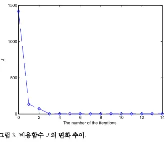
0 2 4 6 8 10 12 14
0 500 1000 1500
The number of the iterations J
3. .
Fig. 3. The cost versus iterations.
.
2 .
4 .
4 , ′, , , ′,
.
5 .
0 0.5 1 1.5 2 2.5 3
0 500 1000
day
0 0.5 1 1.5 2 2.5 3
0 500 1000
day
( )i
x t 측정 오차 20%
측정 오차 0%
측정 오차 10%
측정 오차 30%
측정 오차 0%
측정 오차 10%
측정 오차 20%
측정 오차 30%
( )i
y t
5.
.
Fig. 5. The estimated states using the estimated parameters in the presence of the different measurement errors at the output.
5
.
.
HIV .
, HIV
.
.
추정한 모델의 평형점 분석 IV.
III
HIV .
HIV .
1)
2) ′ ′
′
′
3) ′ ′
. 20%
(1) .
6
7 .
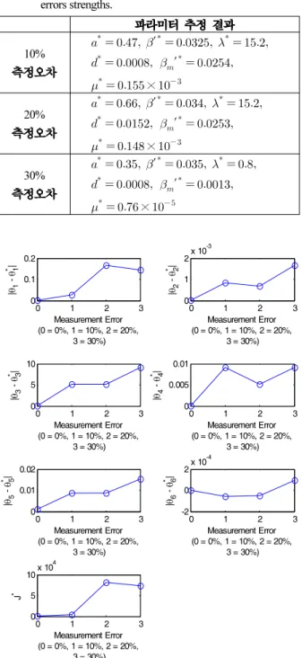
2. .
Table 2. The estimated parameters versus different measurement errors strengths.
10% ′
′
×
20% ′
′
×
30% ′
′
×
0 1 2 3
0 0.1 0.2
Measurement Error (0 = 0%, 1 = 10%, 2 = 20%,
3 = 30%)
|θ1 - θ1
*|
0 1 2 3
0 1 2x 10⁻³
Measurement Error (0 = 0%, 1 = 10%, 2 = 20%,
3 = 30%)
|θ2 - θ2
*|
0 1 2 3
0 5 10
Measurement Error (0 = 0%, 1 = 10%, 2 = 20%,
3 = 30%)
|θ3 - θ3
*|
0 1 2 3
0 0.005 0.01
Measurement Error (0 = 0%, 1 = 10%, 2 = 20%,
3 = 30%)
|θ4 - θ4
*|
0 1 2 3
0 0.01 0.02
Measurement Error (0 = 0%, 1 = 10%, 2 = 20%,
3 = 30%)
|θ5 - θ5
*|
0 1 2 3
-2 0 2x 10⁻⁴
Measurement Error (0 = 0%, 1 = 10%, 2 = 20%,
3 = 30%)
|θ6 - θ6
*|
0 1 2 3
0 5 10x 104
Measurement Error (0 = 0%, 1 = 10%, 2 = 20%,
3 = 30%) J*
4. .
Fig. 4. The estimation errors and the cost versus different measurement errors strengths.
( ) 1 ' 0.53 0.49 e = 1000
x0
31.8
평형점 1 (불안정)
평형점2 (불안정) 15
에이즈 상태
e 평형점 3 (안정)
평형점 2 (안정)
(1000)
(29.9) ( )15
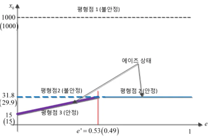
6.
.
Fig. 6. The equilibrium analysis using the estimated parameters in the absence of the measurement error.
( ) 1 ' 0.25 0.49 e = 1000
x0
26.28
평형점 1 (불안정)
평형점2 (불안정) 19.6
에이즈 상태
e 평형점 3 (안정)
평형점 2 (안정)
(1000)
(29.9) ( )15
7. 20%
.
Fig. 7. The equilibrium analysis using the estimated parameters in the presence of the 20% measurement error.
6 7
.
. 6
1
.
.
,
0 .
HIV ( , )
. 2
′ ′ ′
′
′
′′
′ .
10%
AIDS . ( ′
1 2
.)
3
′′ ′.
′ .
10% 0
.
AIDS .
( ′ 1
3
0
.)
( ′),
2 AIDS .
( ′ ), 2
3 AIDS
.
.
7 6 (bifurcation)
′ . ,
.
.
결론 V.
HIV .
.
.
. ,
. ,
, ,
.
참고문헌
[1] M. A. Nowak and C. R. Bangham, “Population dynam- ics of immune responses to persistent viruses,” Science, vol. 272, no. 5258, pp. 74-79, 1996.
[2] M. A. Nowak, S. Bonhoeffer, G. M. Shaw, and R. M.
May, “Anti-viral drug treatment: dynamics of resistance in free virus and infected cell populations,” Journal of Theoretical Biology, vol. 184, pp. 203-217, 1997.
[3] X. Xia, “Estimation of HIV/AIDS parameters”
Automatica, vol. 39, pp. 1983-1988, 2003.
[4] X. Xia and C. H. Moog, “Identifiability of nonlinear systems with applications to HIV/AIDS models,” IEEE Transaction on Automatic Control, vol. 48, no. 2, pp.
330-336, 2003.
[5] S.-K. Kim, C.-N. Kim, and T.-W. Yoon, “Output feed- back parameter estimation for a HIV model with mu- tants,” Proc. of Modelling, Identification, and Control 2011, pp. 399-405, 2011.
[6] R. A. Filter, X. Xia, and C. M. Gray “Dynamic HIV/AIDS parameter estimation with application to a vaccine readiness study in southern africa,” IEEE Transaction on Biomedical Engineering, vol. 52, no. 5, pp. 784-791, 2005.
[7] C. Houck, J. Joins, and M. Kay, “A genetic algorithm for function optimization: a matlab implementation,”
NCSU-IE, TR95-09, 1995.
[8] P. P. Menon, J. Kim, D. G. Bates, and I. Postlethwalte,
“Clearance of nonlinear flight control laws using hybrid evolutionary optimization,” IEEE Transaction on Evolutionary Computation, vol. 10, no. 6, pp. 689-699, 2006.
[9] “Optimization Toolbox User's Guide,” ver.2, The MathWorks, 2000.
[10] H. Bock, “Recent advances in parameter identification for ordinary differential equations,” Progress in Scientific Computing, vol. 2, pp. 95-121, 1983.
[11] K.-R. Cho, S.-W. Baek, and D.-W. Lee, “Fitness change of mission scheduling algorithm using genetic theory ac-
cording to the control constants,” Journal of Institute of Control, Robotics and Systems (in Korean), vol. 16, no.
6, June 2010.
김 석 균 2004
. 2004 ~
․ .
, ,
, ,
. 김 정 수
1998 .
2000 , 2005 , .
2005 ~2008 ,
, Stuttgart ,
Leicester .
. , ,
, , .
윤 태 웅 1984
. 1986 . 1994
. 1995 ~ .
․ .
.
![Fig. 1. The flowchart of the hybrid genetic algorithm [8].](https://thumb-ap.123doks.com/thumbv2/123dokinfo/4696607.505164/3.892.216.681.98.728/fig-flowchart-hybrid-genetic-algorithm.webp)