Contrast Enhancement for Segmentation of Hippocampus on Brain MR Images
Nyamlkhagva Sengee†, Altansukh Sengee††, Enkhbolor Adiya†††, Heung-Kook Choi††††
ABSTRACT
An image segmentation result depends on pre-processing steps such as contrast enhancement, edge detection, and smooth filtering etc. Especially medical images are low contrast and contain some noises.
Therefore, the contrast enhancement and noise removal techniques are required in the pre-processing.
In this study, we present an extension by a novel histogram equalization in which both local and global contrast is enhanced using neighborhood metrics. When checking neighborhood information, filters can simultaneously improve image quality. Most important is that original image information can be used for both global brightness preserving and local contrast enhancement, and image quality improvement filtering. Our experiments confirmed that the proposed method is more effective than other similar techni- ques reported previously.
Key words: contrast enhancement, histogram equalization, neighborhood metrics
※ Corresponding Author : Heung-Kook Choi, Address : (621-749) Injero 197, Gim-Hae, Gyeong-Nam, Korea, Dept. of Computer Engineering, Inje University, Korea, TEL : +82-55-320-3437, FAX : +82-055-322-3107, E-mail
Receipt date : Feb. 7, 2012, Revision date : June 22, 2012 Approval date : Aug. 2, 2012
††††Dept of Computer Engineering, Inje University, Korea (E-mail: [email protected])
††††Dept of Computer Engineering, Inje University, Korea (E-mail: [email protected])
††††Dept of Computer Engineering, Inje University, Korea (E-mail: [email protected])
††††Dept of Computer Engineering, UHRC, Inje University, Korea
※ This research was supported by Basic Science Research Program through the National Research Foundation of Korea (NRF) funded by the Ministry of Education, Science and Technology (2011-0008627)
1. INTRODUCTION
The development of medical imaging tech- nologies in last three decades has grown and enor- mously increased its importance in the diagnosis of diseases. Diagnostic imaging techniques such as ultrasound (US), computer tomography (CT), and magnetic resonance imaging (MRI) facilitate the
recognition of abnormal morphologies as symp- toms of underlying conditions. For instance, hippo- campus morphology has an important role in the earliest stage of Alzheimer’s disease. Hence, hip- pocampus volumetric data has been used as an im- portant biomarker in clinical studies [1-5]. A typi- cal 3D data set is a group of 2D slice images ac- quired by US, CT, and MRI. A good precision and accuracy are required to detect the hippocampus because few slices contain the hippocampus in the slices. Although there are many different segmen- tation approaches, their accuracies are depended on pre-processing steps. Most medical images are low contrast and contain some noises. Therefore, the contrast enhancement and noise removal techni- ques are required in the pre-processing.
In contrast enhancement methods, histogram equalization (HE) is the most well-known techni- que because of its simplicity and processing speed.
HE can be categorized into two main processes:
global histogram equalization (GHE) and local his- togram equalization (LHE) [6]. In GHE, the histo- gram of the whole input image is used to compute
Fig. 1. a) Original b) result of GHE.
a histogram transformation function. As result, the dynamic range of the image histogram is flattened and stretched, and the overall contrast is improved [7].
GHE is an attractive tool in many contrast en- hancement applications. However, it changes the original image’s brightness, while reducing the quality of the original image and in some cases causes a washout effect (Fig. 1). In contrast, LHE uses a sliding window method, in which local his- tograms are computed from the windowed neigh- borhood to produce a local intensities remapping for each pixel. The intensity of the pixel at the cen- ter of the neighborhood is changed according to the local intensity remapping for that pixel. LHE is ca- pable of producing great contrast results but is sometimes thought to over-enhance images.
To overcome the washout effect, brightness- preserving extensions of GHE have been devel- oped, such as brightness-preserving bi-histogram equalization (BBHE) [8], dualistic sub-image his- togram equalization (DSIHE) [9], minimum mean brightness error bi-histogram equalization (MM- BEBHE) [10] and other methods [11-17]. All of the methods mentioned above feature the same weak- ness: they have not considered the enhancement of noisy images and the image visualization is not enhanced on some images that have the histo- grams with a few large bins containing most of the information in the input image.
Eramian [18] generalized the GHE method, which allows any number of neighborhood metrics on image pixels in place of the pixel. The neighbor- hood metric defines a set of temporary sub-bins.
This allows one to choose neighborhood metrics that can order pixels using different criteria and to separate pixels that would be in the same bin in the original histogram into several sub-bins de- fined by neighborhood metric (Fig 2). However all previous works can not remove noise with contrast enhancement simultaneously.
For this reason, we proposed a new extension of GHE which uses distinction neighborhood met- ric [19] for improving contrast and rearranges his- togram for removing noise in this work.
This paper is organized as follows. Related works are discussed in section IIand proposed method is presented in section. Section IV contains some results and comparison between our method and other methods. Section V is our conclusions and further works.
Fig. 2. Demonstration of the neighborhood metric.
2. RELATED WORKS
2.1 Global histogram equalization
Let be the i-th bin of intensity level of origi- nal image , and then is the probability that the gray level of any given pixel is ≤ ≤ :
for (1)
and (2)
where is the number of pixels of i-th intensity level in image , N is the total number of pixels
of image , and L is discrete intensity level. The cumulative distribution function (CDF) is de- fined by (3):
(3)
GHE maps the original image into the resultant image using the intensity transformation function:
(4)
where and are the original and resultant im- ages, are the 2D coordinates of the images, and T is the intensity transformation function, which maps the original image into the entire dy- namic range and ∈ , using CDF:
· (5)
2.2 Bi-histogram equalization (BBHE)
Let be the mean of the image and assume that ∈ . Based on , the image is sepa- rated into two sub-images and as
∪
(6)
where
≤ ∀ ∈ (7) and
∀ ∈ (8) Note that sub-image is composed of { } and the sub-image is composed of { }.
Next, define the respective probability dis- tribution functions of sub-images and as
(9)
and
(10)
in which
and
(where k=0,1,..., and k=
, ,..., correspondingly) represent the respective values of in the two sub-images
and , and
and
are the total values of
and respectively. Here,
,
, and . The respective CDFs are then defined as
(11)
and
(12)
Note that and by definition.
Let us similarly define the following trans- formation functions exploiting the CDFs
·
(13)
and
·
(14)
Then the resultant image of the histogram can be expressed as
(15)
in which
· · i f≤ (16)
2.3 Histogram equalization with neighbor hood metric (HENM)
Let r be sub-bins of the i-th bin, h(i), of in- tensity level of image f and r is produced by a neighborhood metric. The number of total sub-bins is R which equals r· and the range of r depends on the chosen neighborhood metrics.
for (17)
and (18)
Fig. 3. Illustration of the neighborhood metric and filtering in a histogram bin. Pixels of equal intensity are arranged into a) sub-bins using neighborhood information and b) sub-bins using neighborhood information with filtering.
where is the number of occurrences of the r-th sub-bin in i-th intensity of image f and N is the total number of pixels in image f. Then the CDF,
, is defined by (19):
(19)
GHE maps the original image into the resultant image using the intensity transformation function:
(20)
where f and g are the original and resultant images, (x, y) are the 2D coordinates of the images, and
is the intensity transformation function, which maps the original image into the entire sub-bin’s range, [ ] and ∈ using CDF:
· (21) here
· (22)
3. PROPOSED METHOD
In the proposed method, the image histogram is divided into two sub-histograms to preserve the image brightness and each histogram bin of each sub-histogram is divided by a distinction metric into sub-bins [19]. Filtering of any drawbacks dur- ing the enhancement of image contrast requires re- arrangement of the histogram when checkingthe neighborhood metric (Fig. 3). This rearrangement is described below, and all filter types are possible.
To check all image pixels that have been neigh- bors, it is necessary to extend the input image.
3.1 Neighborhood metric
Let be the function that extends an image function surrounded by a "background" of zero in- tensity:
∈ ×
(23)
in which an image is N pixels by M pixels in size
and g(x,y) is the intensity of image pixel (x,y). The distinction metric is expressed by the following formula:
′′∈
′′ (24)
which requires the following distinction function:
′′ ′′ ′′
(25)
in which the distinction metric, , is defined by
, the set of pixels forming a square in the
by square neighborhood centered (x,y) on and is positive odd integer.
3.2 Histogram arrangement
When making histogram, we compute both dis- tinction metric and mean value of current pixels and its neighbors. While distinction metric defines current pixels subbins location of its histogram bin, current pixels intensities are changed by their mean value of neighbors (See Fig. 3).
This rearrangement equals noise removal filter.
However, it differs in that its distinction metrics are computed using the original image data. If we use the filtering process first, the distinction met- rics that are computed as the changed neighbors of the filtered image and sub-bins created by the
distinction metric do not use the original neighbor- hood information of the input image. Therefore, the histogram arrangement is performed with simulta- neous computation of the neighborhood metric and filtering computations.
3.3 Bi-histogram equalization with neighbor- hood metric
The number of total sub-bins are R-1, which equals r·. Denote the mean of the image f by
and ∈ . based on , the image is separated into two sub-image and as
∪
(26)
where
≤ ∀ ∈ (27) and
∀ ∈ (28) Next, define the respective probability density functions of sub-images and as
(29) and
(30)
in which
and
(where k=0,1,..., and k=
, ,..., correspondingly) represent the respective values of in the two sub-images
and , and and are the total values of
and respectively. Here, ,
, and , N is the total number of pixels in image f. The respective CDFs are then defined as
(31) and
(32)
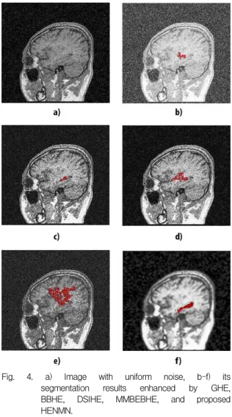
Fig. 4. a) Image with uniform noise, b-f) its segmentation results enhanced by GHE, BBHE, DSIHE, MMBEBHE, and proposed HENMN.
Note that and by definition.
Then the resultant image of the histogram can be expressed as (20)
in which f and g are the original and resultant images, (x,y) are the 2D coordinates of the images, and is the intensity transformation function, which maps the original image into the entire sub-bin’s range, z, using CDF:
· (33) where
· · i f ≤ (34)
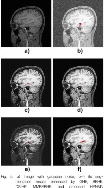
Fig. 5. a) Image with gaussian noise, b-f) its seg- mentation results enhanced by GHE, BBHE, DSIHE, MMBEBHE, and proposed HENMN and filtered by gaussian filter sequentially.
Table 1. Template Matching Fitting percent (%)
Methods Image I Image II
GHE 17 15
BBHE 38 11
DSIHE 24 9
MMBEBHE 16 10
FHENM 93 55
4. EXPERIMENTAL RESULTS
We tested our proposed HENMN method on MRI Brain images which are acquired by GE 3.0T MRI of Inje University Haeundae Paik Hospital, Korea. We present the results of experiments com- paring the proposed method to GHE, BBHE, DSIHE, and MMBEBHE. In the experiment, we tested the proposed method on two different patient images effected by uniform and Gaussian noises comparing to GHE, BBHE DSIHE and MMBEBHE methods.
Fig. 4 shows that the brain image is effected the uniform noise and then improved by different con- trast enhancement methods. Region growing method is used for the hippocampus segmentation and all results are failed except our proposed method's result. As shown Fig. 4, our proposed mehtod is more effective than other existing methods because it used two preprocessing meth- ods simultaneously: filtering and contrast en- hancement. In this experiment, we used mean fil- ter because it is commonly used uniform noise re- moval applications.
It is possible to do sequentially filtering techni- que then contrast enhancement method however, it has two advantages: Our experimental results confirmed that this does not increase the compu- tational cost because the filtering process is done by our proposed arrangement of making the histo- gram while checking neighborhood metrics simultaneously. If the two methods, i.e., histogram equalization and filtering, are performed sequen- tially, the first method uses the original image da- ta and next method uses the data altered by the first. With combined histogram equalization and filtering, the original data can be used for both method Fig. 5 illustrates that original image is ef- fected by gaussian noise and then improved by comparing enhancement methods. Then also they are filtered by gaussian filter for all enhanced images.
Table 1 shows that the fitting percent between the expert and segmentation methods. We can easily see that our proposed contrast enhancement method can remove the noise effectively and its segmentation results is more correctly than other compared methods results.
5. CONCLUSION
In this work, we proposed a new contrast en- hancement method to extract morphological struc- ture of the hippocampus which is difficult to seg- ment due to similarity of surrounding intensities.
The proposed HENMN can improve image con- trast and remove noise simultaneously. Our ex- periment proves that HENMN was very effective pre-processing when segmenting hippocampus using region growing segmentation method. In near future we focus on improvement of segmen- tation accuracy by testing other segmentation method and checking filter etc, because we tested mean filter in this work.
REFERENCES
[ 1 ] H. Wang, J.W. Suh, S. Das, M. Altinay, J.
Pluta, and P. Yushkevich, “Hippocampus Segmentation using a Stable Maximum Likelihood Classifier Ensemble Algorithm,”
Biomedical Imaging: From Nano to Macro, IEEE International Symposium, pp.
2036-2040, 2011.
[ 2 ] Yan Xia, Keith Bettinger, Lin Shen, and Allan L. Reiss., “Automatic Segmentation of the Caudate Nucleus From Human Brain MR Images,” IEEE Transactions on Medical Imaging, Vol. 26, No. 4, pp. 509-517, 2007.
[ 3 ] J. Barnes, J. Foster, R.G. Boyes, T. Pepple, E.K. Moore, J.M. Schott, C. Frost, R.I. Scahill, and N.C. Fox., “A Comparison of Methods for the Automated Calculation of Volumes and Atrophy Rates in the Hippocampus,” Neuro- Image, Vol. 40, No. 4, pp. 1655-1671, 2008.
[ 4 ] Killiany. R.J., Hyman, N., and Gomez-Isla. T.,
“MRI Measures of Entorhinal Cortex vs Hip- pocampus in Preclinical AD,” Neurology, Vol. 58, No. 8, pp. 1188-1196, 2002.
[ 5 ] Xu. Y., Jack Jr. C.R., O’Brien. P.C., Kokmen.
E., Smith. G.E., Ivnik. R.J., Boeve. B.F., Tan-
galos. R.G., and Petersen. R.C., “Usefulness of MRI Measures of Entorhinal Cortex Versus Hippocampus in AD,” Neurology, Vol. 54, No.
9, pp. 1760-1767, 2000.
[ 6 ] Sengee. N., Sengee. A., and Choi, H-K,
“Image Contrast Enhancement using Bi-His- togram Equalization with Neighborhood Metrics,” IEEE Transactions on Consumer Electronics, Vol. 56, No. 4, pp. 2727-2734, 2010.
[ 7 ] R. C. Gonzalez and R. E. Woods, Digital Image Processing, Prentice-Hall, New Jersey, 2002.
[ 8 ] Yeong-Taeg Kim, “Contrast Enhancement using Brightness Preserving Bi-histogram Equalization,” IEEE Transactions on Consu- mer Electronics, Vol. 43, No. 1, pp. 1-8, 1997.
[ 9 ] Y. Wang, Q. Chen, and B. Zhang, “Image En- hancement Based on Equal Area Dualistic Sub-image Histogram Equalization Method,”
IEEE Transactions on Consumer Electronics, Vol. 45, No. 1, pp. 65-75, 1999.
[10] S.D. Chen and A.R Ramli, “Minimum Mean Brightness Error Bi-histogram Equalization in Contrast Enhancement,” IEEE Transactions on Consumer Electronics, Vol. 49, No. 4, pp.
1310-1319, 2003.
[11] S.D. Chen and A.R Ramli, “Contrast Enhance- ment using Recursive Mean-separate Histo- gram Equalization for Scalable Brightness Preservation,” IEEE Transactions on Consu- mer Electronics, Vol. 49, No. 4, pp. 1301-1309, 2003.
[12] K.S. Sim, C.P. Tso, and Y.Y. Tan, “Recur- sive Sub-image Histogram Equalization Ap- plied to Gray Scale Images,” Pattern Recog- nition Letters, Vol. 28, No. 10, pp. 1209- 1221, 2007.
[13] D. Menotti, L. Najman, J. Facon, and A.D.A.
Araujo, “Multi-Histogram Equalization Me- thods for Contrast Enhancement and Bright- ness Preserving,” IEEE Transactions on
Consumer Electronics, Vol. 53, No. 3, pp.
1186-1194, 2007.
[14] A.A. Wadud, M.H. Kabir, M.A.A. Dewan, and O. Chae, “A Dynamic Histogram Equaliza- tion for Image Contrast Enhancement,” IEEE Transactions on Consumer Electronics, Vol.
53, No. 2, pp. 1-2, 2007.
[15] H. Ibrahim and N.S.P. Kong, “Brightness Preserving Dynamic Histogram Equalization for Image Contrast Enhancement,” IEEE Transactions on Consumer Electronics, Vol.
53, No. 4, pp. 1752-1758, 2007.
[16] S.M. Pizer, E.P. Amburn, J.D. Austin, R.
Cromartie, A. Geselowwitz, T. Greer, B.H.
Romeny, J. B. Zimmerman, and K. Zuiderveld,
“Adaptive Histogram Equalization and Its Variations,” Computer Vision, Graphics, and Image Processing, Vol. 39, No. 3, pp. 355-368, 1987.
[17] C. Wang and Z. Ye, “Brightness Preserving Histogram Equalization with Maximum Entropy: A Variational Perspective,” IEEE Transactions on Consumer Electronics, Vol.
51, No. 4, pp. 1326–1334, 2005.
[18] M. Eramian and D. Mould, “Histogram Equal- ization using Neighborhood Metrics,”
Proceedings of Computer and Robot Vision, the 2nd Canadian Conference on IEEE CNF, pp. 397-404, 2005.
[19] Sengee. N and Choi. H-K, “Contrast En- hancement using Histogram Equalization with a New Neighborhood Metrics,” Journal of Korea Multimedia Society, Vol. 11, No. 6, pp. 737-745, 2008.
Nyamlkhagva Sengee
2003. 8 B.S. National University Mongolia, Mongolia 2008. 3 M.S. Inje University,
Korea
2012. 8. Ph.D. Inje University, Korea
Research Fields : Computer Graphics, Image Processing
Altansukh Sengee
2006. 8 B.S. National University Mongolia, Mongolia 2012. 8 Graduate Student, Inje
University, Korea Research Fields : Computer
Graphics, Image Processing
Enkhbolor Adiya
2004. 8 B.S. National University Mongolia, Mongolia 2006. 8 M.S. National University
Mongolia, Mongolia 2012. 8 Ph.D. Student, Inje
University, Korea Reaearch Fields: Image Pro- cessing and Analysis
Heung-Kook Choi
1988. 8 B.S. Linköping Univ.
Sweden
1990. 8 M.S. Linköping Univ.
Sweden
1996. 9 Ph.D. Uppsala Univ.
Sweden
Research Fields: Computer Graphics, Image Processing