Review of low-noise radio-frequency amplifiers based on superconducting quantum interference device

(1)

Progress in Superconductivity and Cryogenics

Vol.16, No.4, (2014), pp.1~6 http://dx.doi.org/10.9714/psac.2014.16.4.001

```

1. INTRODUCTION

Superconducting quantum interference device (SQUID) is a sensitive detector of magnetic flux signals. Until now, SQUIDs were mainly used to measure signals in the frequency range from near DC to few MHz using the flux-locked loop (FLL) circuits. In FLL operation, the measurement bandwidth is limited due to gain-bandwidth product of room-temperature electronics and time delay from the feedback circuits and the signal lines. However, if the SQUID is operated in open loop with input flux amplitude smaller than half flux quantum and fast signal cables were used, we can measure high-frequency signals.

Recently, there were several reports on the development of SQUID amplifiers operating in the radio-frequency (RF) range, that is, from 200 MHz up to 10 GHz. One use of this SQUID RF amplifier is to detect axion-mediated weak RF signals from a cryogenic microwave cavity [1]. For example, in the project of Axion Dark Matter eXperiment (ADMX), the operating frequency was below 1 GHz, and recently ADMX team plans to increase the frequency.

The other application of SQUID RF amplifiers is to detect quantum-bit signals in quantum information processing experiments. In this case, the operating frequency is about from 4 GHz to 8 GHz [2].

In either application of SQUID RF amplifiers, key performance factors are operating frequency, power gain, bandwidth and noise temperature. Here, we reviewed SQUID RF amplifiers developed at several groups, compared their designs and performances, and predict future development direction for improved gain and noise temperature at higher frequencies.

* Corresponding author: [email protected]

2. BASIC PRINCIPLE OF SQUID RF AMPLIFIER 2.1. Configuration of SQUID RF Amplifier

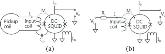
SQUID sensors for measuring low-frequency signals have input coil integrated on top of the SQUID loop with the two ends of the input coil connected to the pickup coil as shown in Fig. 1(a). In the high frequency range, the parasitic capacitance Cp between the input coil and SQUID loop increases, and this makes the transfer of input flux into SQUID loop difficult. By placing the input coil inside the SQUID hole, the parasitic capacitance can be reduced much, but the multi-turn coil inside the SQUID hole reduces the mutual inductance with the SQUID loop, resulting in reduction of the amplifier gain [3, 4].

One idea of circumventing the parasitic capacitance effect is to use it. M. Mück and J. Clarke made a microstrip structure of the input coil, in which the input coil forms a microstrip with one end of it is left open and the input signal is applied between the other end of it and the ground as shown in Fig. 1(b) [5, 6].

(a) (b)

Fig. 1. Structure of DC-SQUIDs. (a) Typical DC-SQUID magnetometer for measuring low-frequency magnetic fields, and (b) DC-SQUID amplifier for measuring RF signals where one end of the input coil is left open.

Review of low-noise radio-frequency amplifiers based on superconducting quantum interference device

Y. H. Lee^{*, a}, Y. Chong^b, and Y. K. Semertzidis^c

a Center for Biosignals, Korea Research Institute of Standards and Science, Daejeon, Korea

b Center for Quantum Measurement Sciences, Korea Research Institute of Standards and Science, Daejeon, Korea

c Center for Axion and Precision Physics Research, Institute for Basic Science, Daejeon, Korea (Received 18 December 2014; revised 29 December 2014; accepted 30 December 2014)

Abstract

Superconducting quantum interference device (SQUID) is a sensitive detector of magnetic flux signals. Up to now, the main application of SQUIDs has been measurements of magnetic flux signals in the frequency range from near DC to several MHz.

Recently, cryogenic low-noise radio-frequency (RF) amplifiers based on DC SQUID are under development aiming to detect RF signals with sensitivity approaching quantum limit. In this paper, we review the recent progress of cryogenic low-noise RF amplifiers based on SQUID technology.

Keywords: SQUID, Cryogenic amplifier, RF signal measurement, Noise temperature

(2)

Review of low-noise radio-frequency amplifiers based on superconducting quantum interference device

(a)

(b)

Fig. 2. Cross-sectional view of the microstrip line. (a) Side view showing the vertical structure, and (b) end view showing the layout of input coil on SQUID washer.

When an input RF signal Vi is applied to the input coil, a standing wave electric field is generated in the microstrip line, and its resonance frequency is determined by several parameters of the device. Finally, the magnetic flux from the current Ii is focused into the SQID hole and converted into output voltage Vo. This scheme of SQUID RF amplifier is called a microstrip SQUID amplifier (MSA).

The structure of the MSA in thin film type is shown in Fig. 2. Two superconducting thin films are separated by a dielectric layer of thickness d and dielectric constant ε. The multi-turn input coil has a linewidth w. Assuming that the thickness of two superconducting films are much thicker than the London penetration depth of the superconductor λ and w>>d, the capacitance and inductance per unit length of the microstrip are respectively given as following,

C0=εε0w/d (F/m), (1) L0=(μ0d/w)(1+2λ/d) (H/m), (2) where, ε0 and μ0 are permittivity and permeability in vacuum. The velocity of an electromagnetic wave in the microstrip is then given by

c^*=1/(L0C0)^1/2=c/[ε(1+2λ/d)]^1/2, (3) where, c is the velocity of light in vacuum. Finally the characteristic line impedance of the microstrip is given by

Z0=(L0/C0)^1/2=(d/w)[μ0(1+2λ/d)/εε0]^1/2. (4) 2.2. Performance parameters of SQUID RF Amplifier 2.2.1. Resonance frequency

When the microstrip has length l, and its ends are open with source resistance Ri(>Z0), it becomes a half-wave resonator with its wavelength given by the relation, l=λ/2.

And the quality factor of the resonator is Q=πRi/2Z0. Since Z0 can be made to be smaller than Ri, Q can be larger than 1.

Then, the resonance frequency f0(L0) of the microstrip is given by,

f0(L0)=c^*/λ=c^*/2l=1/2l(L0C0)^1/2=c/2l(ε(1+2λ/d))^1/2. (5) The expression for the resonance frequency (Eq. 5) agrees with the experimental values in the frequency range of below few hundreds MHz. With the increase of frequency, however, Eq. (5) deviates much from the measured ones. For example, at 2 GHz, measured one is about 5 times smaller than given by Eq. (5) [7].

As l becomes shorter for higher frequencies, parasitic inductance becomes important and thus the effective length increases, resulting in decreased resonance frequency. In practical assembly of the device, low-inductance wiring is needed by using short and parallel bonding wires between RF input pad in the printed circuit board and microstrip input coil pad in the SQUID chip.

Considering that the flux signal into the SQUID loop is transferred through the input coil, the actual inductance of the microstrip also can be estimated from the input coil inductance with its resonance frequency given by,

f0(n²LSQ)=c^*/2l=1/2l(L0*C0)^1/2=1/2n(lLSQC0)^1/2, (6) where, L0*=Li/l=n²LSQ/l is inductance of the input coil per unit length, l input coil length, n number of input coil turn and LSQ SQUID inductance. This input coil resonance frequencies were shown to be about 2 times larger than measured ones, and thus Eq. (6) agrees with experimental values better than Eq. (5) in the GHz range.

2.2.2. Gain of the MSA

In typical applications of DC-SQUIDs, flux-locked loop operation is used to linearize the SQUID response against input flux signals, with maximum measurement frequency range of about 10 MHz. In the RF frequency, for example, GHz range, one has to operate the SQUID in open loop mode. When a small input voltage signal Vi (as shown in Fig. 1 (b)) is applied to the input circuit with impedance Ri, then the current Ii=Vi/Ri generates magnetic flux into SQUID loop given by Φ=IiMi. The SQUID output voltage Vo of the SQUID becomes (Vi/Ri)MiVΦ, with VΦ the flux-to-voltage transfer coefficient of the SQUID. The voltage gain is then (Vo/Vi)=MiVΦ/Ri.

To calculate the power gain, one has to take into account the impedance ratio, and then the power gain is given by,

G=(Vo/Vi)²(Ri/Z0)=~Mi2VФ2. (7) Since Mi is roughly nLSQ, with n the number of input coil turns, and VФ is approximately R/LSQ=~(πLSQC)^-1/2, with R the SQUID dynamic resistance and C the junction effective capacitance, G is proportional to n²LSQ. That is, larger number of turns for the input coil is desirable while keeping the total length of the microstrip and inductance of the input coil kept constant to have a required resonance frequency.

2

(3)

Y. H. Lee, Y. Chong, and Y. K. Semertzidis

2.2.3. Noise temperature

Experimentally, the noise temperature of the MSA is given by,

TN= ~ f0T/VФ ~ f0TLSQ1/, (8) where, f0 is the resonance frequency and T is the bath temperature. To have lower noise temperature, larger VФ is needed as in the amplifier gain. Physically, cooling the MSA device to as low temperature as possible is needed.

3. SEVERAL MSA DEVELOPMENTS 3.1. University of California at Berkeley (UC Berkeley)

The operating frequency range of the MSAs developed in the UC Berkeley was from about 200 MHz to 7.6 GHz.

The resonance frequency could be controlled rather easily by changing the length of the microstrip. In a SQUID having inner dimensions of 0.2 mm × 0.2 mm and SQUID inductance of 320 pH, for example, the resonance frequency changes with microstrip length l as 1.49 × 104/(l+16) MHz [5]. The power gains were about 20 dB at below 1 GHz, but they decrease at higher frequencies than about 1 GHz as shown in Fig. 3.

In an MSA having cooling fins to cool the hot electrons in the shunt resistors, they reported noise temperature of about 48 mK operated at 612 MHz, which is within a factor of 1.6 of the quantum limit, as shown in Fig. 6 [8]. In the MSAs of UC Berkeley, the design variations are in the SQUID loop size, number of input coil turns and linewidth of the input coil.

Fig. 3. Gain-frequency curves for 6 MSAs having different SQUID loop sizes and input coil lengths. Numbers are coil lengths in mm [7].

Fig. 4. Noise temperature vs bath temperature. TQ is the quantum limit TQ=hf/kB with h Planck constant, f frequency and kB Boltzmann constant [8].

(a)

(b)

Fig. 5. Frequency tuning using a varactor. (a) Configuration of MSA with a varactor connected between one end of the microstrip and ground. (b) Gain vs frequency for 9 different bias voltages applied to the varactor [9].

3.1.1. Tuning of the resonance frequency

The resonance frequency of the MSA can be tuned by connecting a variable capacitor (varactor) to one end of the microstrip. The frequency can be reduced in-situ by ~ 40 % from the original (maximum) frequency by changing the capacitance between the input and ground (Fig. 5) [9]. But, it is not possible to increase the frequency by this scheme.

3.1.2. Cascade amplifier (two-stage amplifier)

By connecting a second amplifier to the first amplifier with a circulator in between them, the overall performance of the MSA chain can be improved. The bandwidth of the MSA chain can be increased if the two frequencies are slightly detuned. And, if the two frequencies overlapped, gain at the center frequency can be increased much (Fig. 6).

Fig. 6. Two-stage MSA chain. (a) Gain vs frequency with two frequencies detuned slightly to increase bandwidth, and (b) two frequencies coincide each other to increase gain at the overlapped center frequency [9].

3

(4)

3.2. Syracuse University

Both the amplifier gain and noise temperature can be improved by increasing the flux-to-voltage transfer VФ, which can be increased by increasing the shunt resistance of the SQUID while keeping the Stewart-McCumber parameter βc(=2πI0R²CJ/Ф0) less than 1, with I0 , R and CJ

the critical current, shunt resistance and effective capacitance of one junction, respectively, and Ф0 the flux quantum. Thus, small-sized junctions with small parasitic capacitance can allow large R. In the Syracuse University, they used an electron beam lithography and shadow evaporation method to fabricate sub-μm junctions with a junction area of 0.73 μm × 0.18 μm. As shown in Fig. 7, flux-voltage curves are quite steep against magnetic flux and VФ value is about 3 mV/Ф0.

The aluminum input coil has a linewidth of 5 μm, 16 turns and total length of 8.3 mm. The measured gain is as high as 32 dB at 1.55 GHz. For the other series of MSAs, as shown in Fig. 8, with a higher resonance frequency of 3.8 GHz, the gain and bandwidth are G=17 dB and 150 MHz, respectively. Noise temperature measured at 3.8 GHz is 0.55±0.13 K at bath temperature of 0.35 K. Considering that the quantum limit of 3.8 GHz is 0.18 K, the measured system noise temperature is nearly the same as the sum of bath temperature and quantum limit. The authors suggested that the noise temperature is limited by the hot electrons in the shunt resistors. Thus, if cooling fins are added, the noise temperature could be reduced.

Fig. 7. Flux-voltage curves of the DC-SQUID amplifier for different bias currents fabricated using sub-μm Al/AlOx/Al junctions [10].

Fig. 8. Structure of the MSA in Syracuse University in different microscopic scales. (a) Input part with a coupling capacitor, (b) input coil, (c) shunt resistors, (d) junction area, and (e) junctions [11].

3.3. National Institute of Standards and Technology(NIST) In the NIST, the main motivation for developing the MSA was to readout superconducting qubit signals.

Lumped element design method was applied for modular evaluation and development of each component, including coupling capacitor and inductor (Fig. 9). Four-hole gradiometric type SQUID washer was used to have low SQUID inductance and to keep the coupling of RF signal into SQUID loop at high frequency [12, 13].

The target frequencies were 1~8 GHz range. At 1.7 GHz, typical gains were about 20 dB, and maximum gain was about 30 dB in one device. In the range 5~7 GHz, the gains were 15~20 dB. As shown in Fig. 10(a), there is a trade-off between gain and bandwidth. In one device, the gain-bandwidth product was as large as 27 GHz and bandwidth of over 1 GHz (Fig. 10(b). In general, the gain curves show complex frequency dependence due to the complex feedback effects of the SQUID. Noise temperature was below 1 K (3 photons of added noise) at in the frequency range 4~8 GHz at 30 mK.

Fig. 9. Structure of MSA with lumped element design. (a) Overall device layout, (b) part of coupling circuit, and (c) detailed structure of SQUID part [13].

Fig. 10. Gain curves in two MSAs. (a) Gains at different flux biases, (b) gain in a different device with a bias point for high bandwidth, and (c) same bias point as (b) [13].

4

(5)

Y. H. Lee, Y. Chong, and Y. K. Semertzidis

4. SLUG AMPLIFER

4.1. SLUG RF amplifier at University of Wisconsin MSA needs a multi-turn input coil and the gain is proportional to the number of turns of the input coil, which limits the gain at high frequencies. An effective method to couple high-frequency signals into SQUID is an amplifier based on superconducting low-inductance undulatory galvanometer (SLUG), which is a variation of DC-SQUID.

In SLUG, RF signal is coupled directly into the SQUID loop as a current instead of flux. Thus, input coil is not needed. A structure of the SLUG design in the University of Wisconsin, Madison, is shown in Fig. 11 [14].

The gains were 25 dB at 3 GHz and 15 dB at 9 GHz, and bandwidth of several hundred MHz (Fig. 12). However there is no measurement data on the noise temperature.

SLUG also has shunt resistors as in the DC-SQUIDs, thus cooling fins are needed to cool the hot electrons for lower noise temperature [16].

Fig. 11. RF amplifier based on SLUG. (a) Vertical side view, (b) top-down view, and (c) schematic diagram of the SLUG RF amplifier [15].

Fig. 12. Gain curves of a SLUG amplifier at different flux bias points. (a) Gain at the first resonant mode and (b) second resonant mode [15].

Since input signal is directly connected to SLUG as a current, the possibility of device damage due to electrostatic discharge is higher than DC-SQUID, thus care should be taken in handling the devices.

5. FUTURE TREND OF DEVELOPMENT 5.1. Amplifier gain at high frequencies

Gain is approximately proportional to the product of turn number of input coil n and flux-to-voltage transfer VΦ. To decrease n, smaller SQUID hole dimensions and narrow-linewidth for input coil can be applied. To increase VΦ, smaller SQUID inductance and smaller junction size to allow larger shunt resistance are possible. In decreasing SQUID inductance, SLUG could be a solution.

5.2. Noise temperature

Noise temperature improves by increasing VΦ, as in the amplifier gain. When shunt resistors are used, cooling fins should be used to cool the hot electrons in the resistors.

6. SUMMARY

Design of MSAs at University of California, Berkeley, showed sufficient gains at frequencies below 1 GHz, but the gain drops much from frequency above about 2 GHz.

The noise temperature at 600 MHz with cooling fins approached near the quantum limit. But, the latest designs of UC, Berkeley did not improve much from its original standard MSA type.

In Syracuse University with submicron-sized junctions resulted in large flux-to-voltage transfer, and improved gain, e.g., 17 dB at 3.8 GHz, and noise temperature is 0.55 K without cooling fins. The input coil design is not much changed from the UC, Berkeley’s design.

In the approach of NIST, small-inductance SQUID and quarter-wave resonator was used to enhance the RF coupling to the SQUID. The gains are comparable to those of Syracuse’s results. But, noise temperatures were not reported yet. If submicron junctions are used in the design of NIST, improved performance in the gain and noise temperature would be possible.

SLUG has an advantage of direct coupling of RF signal into SQUID as a current input, and the amplifier based on SLUG can be operated up to about 10 GHz with moderate gains.

Since both microstrip SQUID amplifier and SLUG amplifier are improving in performance, improved design or combination of different design will improve the performances further.

ACKNOWLEDGMENT

This work was supported by IBS project of CAPP.

5

(6)

REFERENCES

[1] S. J. Asztalos et al., “Design and performance of the ADMX SQUID-based microwave receiver,” Nucl. Instr. Meth. Phys. Res., A 656, pp. 39-44, 2011.

[2] S. Michotte, “Qubit dispersive readout scheme with a microstrip superconducting quantum interference device amplifier,” Appl.

Phys. Lett., vol. 94, pp. 122512-1~3, 2009.

[3] M. A. Tarasov, V. Yu. Belitsky and G. V. Prokopenko, “DC SQUID RF Amplifiers,” IEEE T. Appl. Supercond., vol. 2, pp. 79-83, 1992.

[4] G. V. Prokopenko, S. V. Shitov, V. P. Koshelets, D. B. Balashov, and J. Mygind, “A dc SQUID based low-noise 4 GHz amplifier,”

IEEE T. Appl. Supercond., vol. 7, pp. 3496-3499, 1997.

[5] J. Clarke, M. Mück, M. André, J. Gain and C. Heiden, “The Microstrip DC SQUID Amplifier,” pp. 473-504, in Microwave Superconductivity, Eds. H. Weinstock and M. Nisenoff, 2001, Kluwer Academic Pub.

[6] M. Mück, and J. Clarke, “The superconducting quantum interference device microstrip amplifier: Computer models,” J.

Appl. Phys., vol. 88, pp. 6910-6918. 2000.

[7] J. Clarke, A. T. Lee, M. Mück and P. L. Richards, “SQUID Voltmeters and Amplifiers,” pp. 22-115, Chap. 8, in The SQUID Handbook, Eds. J. Clarke and A. I. Braginski, 2006, Wiley-VCH.

[8] D. Kinion and J. Clarke, “Superconducting quantum interference device as a near-quantum-limited amplifier for the axion dark-matter experiment,” Appl. Phys. Lett., vol. 98, p. 202503, 2011.

[9] M. Mück, M. André, J. Clarke, J. Gail and C. Heiden, “Microstrip superconducting quantum interference device radio-frequency amplifier: Tuning and cascading,” Appl. Phys. Lett., vol. 75, pp.

3545-3547, 1999.

[10] M. P. DeFeo, P. Bhupathi, K. Yu, T. W. Heitmann, C. Song, R.

McDermott, and B. L. T. Pourde, “Microstrip superconducting quantum interference device amplifiers with submicron junctions:

Enhanced gain at gigahertz frequencies,” Appl. Phys. Lett., vol. 97, pp. 092507-1~3, 2010.

[11] M. P. DeFeo, and B. L. T. Pourde, “Superconducting microstrip amplifiers with sub-Kelvin noise temperature near 4 GHz,” Appl.

Phys. Lett., vol. 101, pp. 052603-1~4, 2012.

[12] L. Spietz, K. Irwin, and J. Aumentado, “Input impedance and gain of a gigahertz amplifier using a dc superconducting quantum interference device in a quarter wave resonator,” Appl. Phys. Lett., vol. 93, pp. 082506-1~3, 2008.

[13] L. Spietz, K. Irwin, and J. Aumentado, “Superconducting quantum interference device amplifiers with over 27 GHz of gain-bandwidth product operated in the 4-8 GHz frequency range,” Appl. Phys. Lett., vol. 95, pp. 092505-1~3, 2009.

[14] G. J. Ribeill, D. Hover, Y. –F. Chen, S. Zhu, and R. McDermott,

“Superconducting low-inductance undulatory galvanometer microwave amplifier: Theory,” J. Appl. Phys., vol. 110, pp.

103901-1~13, 2011.

[15] D. Hover, Y. -F. Chen, G. J. Ribeill, S. Zhu, S. Sendelbach, and R.

McDermott, “Superconducting low-inductance undulatory galvanometer microwave amplifier,” Appl. Phys. Lett., vol. 100, pp.

063503-1~3, 2012.

[16] F. C. Wellstood, C. Urbina, and J. Clarke, “Hot-electron effects in metals,” Phys. Rev. B, vol. 49, pp. 5942-5955, 1994.

6