논문 2012-49SC-3-1
데이터 연관 문제와 지능시스템에서의 응용: 리뷰
( Data Association and Its Applications to Intelligent Systems: A Review )
오 성 회**s ( Songhwai Oh )
요 약
데이터 연관은 지능시스템의 자율적인 작동에 매우 중요한 문제이다. 본 논문에서는 데이터 연관 문제를 Bayesian 방식으 로 구성하고 이를 성공적으로 지능시스템에 응용한 예를 설명한다. 먼저 데이터 연관 문제가 어떻게 Bayesian 방식으로 구성 하여 혼잡한 환경에서의 다 물체 추적 문제에 적용되는지 알아본다. 그리고 데이터 연관이 지능시스템에 어떻게 응용될 수 있 는지 정체 관리를 이용한 항공 교통 관제, 카메라 네트워크 위치 및 관점 자동 보정, 멀티 센서 퓨젼의 세 가지 예를 이용해 살펴본다.
Abstract
Data association plays an important role in intelligent systems. This paper presents the Bayesian formulation of data association and its applications to intelligent systems. We first describe the Bayesian formulation of data association developed for solving multi-target tracking problems in a cluttered environment. Then we review applications of data association in intelligent systems, including surveillance using wireless sensor networks, identity management for air traffic control, camera network localization, and multi-sensor fusion.
Keywords : Data association, multi-target tracking, intelligent systems
Ⅰ. Introduction
A data association problem was first formally formulated in the field of (radar-based) multi-target tracking. The objective of radar-based target tracking was to determine tracks of multiple moving objects (or targets) from noisy radar scans in a cluttered environment. Examples of data association algorithms include multiple hypothesis tracker (MHT)[2], joint probabilistic data association (JPDA)[2, 26], and recently
* 평생회원, 서울대학교 전기·정보공학부 (Seoul National University)
※ 이 논문은 2010년도 정부(교육과학기술부)의 재원으 로 한국연구재단의 지원을 받아 수행된 기초연구사 업임 (No. 2010-0027155).
접수일자: 2012년4월3일, 수정완료일: 2012년4월12일
developed Markov chain Monte Carlo data association (MCMCDA)[3].
Data association methods developed for multi-target tracking later found their applications in computer vision for solving a correspondence problem[4] and visual tracking[5]. Data association is used to match image features across multiple images for solving structure from motion, multi-view geometry, 3D reconstruction, image registration, and camera calibration; and to match image features against object models or semantic concepts for object recognition or scene understanding[6]. Recently, multi-target tracking itself has received a considerable amount of attention in the computer vision community because the task of tracking
multiple objects in video sequences is an important step towards understanding dynamic scenes.
Simultaneous localization and mapping (SLAM) in mobile robotics is closely related to structure from motion in computer vision. In SLAM, the task of data association is to recognize whether a newly detected landmark (or feature) is a known landmark in the map or a new landmark[7]. While many available SLAM algorithms assume that all observed landmarks have been correctly identified, there is a strong need to handle data association in SLAM and a growing number of algorithms are proposed. But due to variation in object appearance, noisy sensors, and complexity of the environment, data association is still considered as an unresolved problem in SLAM[8].
Data association also appears in many other areas, such as wireless sensor networks[9], information retrieval[10], and even computer network security[11]. Lastly, we note that data association is also closely related to classification, segmentation, and recognition.
In this paper, we first describe the Bayesian formulation of data association for multi-target tracking problems. Then we review applications of data association in intelligent systems. The remainder of this paper is structured as follows. The Bayesian formulation of data association for multi-target tracking is described in Section II. The remaining chapters describe some of applications of data association to intelligent systems: identity management for air traffic control (Section III), camera network localization (Section IV), and multi-sensor fusion (Section V).
Ⅱ. Bayesian Formulation of Data Association
Let ∈ be the duration of surveillance. Let be the number of targets that appear in the surveillance region during the surveillance period.
Each target moves in for some duration
⊂. Notice that the exact values of
and
are unknown. Each target arises at a random position in at
, moves independently around until , and disappears. At each time, an existing target persists with probability and disappears with probability . The number of targets arising at each time over has a Poisson distribution with a parameter where is the birth rate of new targets per unit time, per unit volume, and is the volume of . The initial position of a new target is uniformly distributed over
.
Let → be the discrete-time dynamics of the target which is assumed to be known, where is the dimension of the state variable, and let ∈ be the state of the target at time for . The target moves according to
(1) for where ∈ are white noise processes. The white noise process is included to model non-rectilinear motions of targets. When a target is present, a noisy observation (or measurement) of the state of the target is measured with a detection probability . Notice that, with probability , the target is not detected and we call this a missing observation. There are also false alarms and the number of false alarms has a Poisson distribution with a parameter , where is the false alarm rate per unit time, per unit volume. Let
be the number of observations at time , including both noisy observations and false alarms.
Let ∈ be the -th observation at time for
, where is the dimension of each observation vector. Each target generates a unique observation at each sampling time if it is detected.
Let → be the observation model. Then the observations are generated as follows:
← (2)
그림 1. (a) 측정값 의 예 (원들은 측정값을 나타내고 그 안의 숫자는 측정 시간을 나타낸다.) (b) 를 분활한 의 예
Fig. 1. (a) An example of observations (each circle represents an observation and numbers represent observation times). (b) An example of a partition of .
where ∈ are white noise processes and
is a random process for false alarms and false alarms are distributed uniformly over . We assume that the targets are indistinguishable in this paper, but if observations include target type or attribute information, the state variable can be extended to include target type information as done in [12].
The main objective of the multi-target tracking problem is to estimate ,
, and
≤ ≤ , for , from noisy observations.
Let be all
measurements at time and
≤ ≤ be all measurements from
to . Let be a collection of partitions of
such that, for ∈ , , where is a set of false alarms and is a set of measurements from target for . Note that is also known as a joint association event in literature. See Fig. 1 for an example.
Let be the number of targets at time
, be the number of targets terminated at time and be the number of targets from time that have not terminated at time . Let be the number of new targets at time , be the number of actual target detections at time and be the number of undetected targets. Finally, let
be the number of false alarms.
Using the Bayes rule, it can be shown that the posterior of is:
∝
∝
∙
(3)
where is the likelihood of observations given , which can be computed based on the chosen dynamic and measurement models. For example, the computation of for the linear dynamic and measurement models can be found in [3]. Our formulation of (3) is similar to MHT[13] and the derivation of (3) can be found in [3]. The parameters , , , and have been widely used in many multiple-target tracking applications[2, 13]. Our experimental and simulation experiences show that our tracking algorithm is not sensitive to changes in these parameters in most cases. In fact, we used the same set of parameters for all our experiments.
There are two major approaches to solve the multi-target tracking problem[3]: maximum a posteriori (MAP) and Bayesian approaches. The MAP approach finds a partition of observations such that
is maximized and estimates the states of the targets based on this partition. A Bayesian approach called minimum mean square error (MMSE) finds an estimate which minimizes the expected square error.
For instance, is the MMSE estimate for the state of target . However, when the number of targets is not fixed, a unique labeling of each target is required to find under the MMSE approach.
The Markov chain Monte Carlo data association (MCMCDA) algorithm was recently proposed to solve data association problems arising in multi-target tracking in a cluttered environment[3]. The data association problem is known to be NP-hard[14] and we do not expect to find efficient, exact algorithms.
Unlike MHT and JPDA, MCMCDA is a true approximation scheme for the optimal Bayesian filter;
i.e., when run with unlimited resources, it converges
to the Bayesian solution. As the name suggests, MCMCDA uses Markov chain Monte Carlo (MCMC) sampling instead of enumerating over all possible associations. Single-scan MCMCDA is a fully polynomial randomized approximation scheme for JPDA while multi-scan MCMCDA outperforms MHT
[3].
In the following sections, we show how MCMCDA has been applied to a number of applications in intelligent systems. For the more detailed description cationsMCMCDA algorithm, we refer readers to [3].
Ⅲ. Distributed Tracking and Identity Management
The tracks estimated by a multi-target tracking algorithm are usually used by other applications.
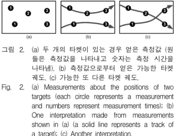
These applications make decisions or reallocate resources based on the estimated tracks, e.g., pursuer assignment and path planning in pursuit-evasion games[9]. But a decision based on a single set of tracks may be risky since tracks do not fully exhibit the uncertainty in the identities of targets accumulated from continuous interactions among crossing or nearby targets. For example, when two targets are moving close to each other, there can be multiple interpretations of the event. Fig. 2(a) shows measurements about positions of two targets over time. Fig. 2(b) and 2(c) shows two possible interpretations made from the measurements shown in Fig. 2(a). Clearly, there can be more than two interpretations due to measurement noise and identity uncertainty but a multi-target tracking algorithm can only display a single interpretation (usually the one with the highest likelihood or an interpretation with expected positions). Since the number of possible interpretations grows exponentially as more measurements are collected, we can not display all possible interpretations. For a networked system such as sensor networks, the communication medium is bandwidth-limited, hence, it is necessary to represent the uncertainty about the identities in the most
그림 2. (a) 두 개의 타켓이 있는 경우 얻은 측정값 (원 들은 측정값을 나타내고 숫자는 측정 시간을 나타냄). (b) 측정값으로부터 얻은 가능한 타켓 궤도. (c) 가능한 또 다른 타켓 궤도.
Fig. 2. (a) Measurements about the positions of two targets (each circle represents a measurement and numbers represent measurement times); (b) One interpretation made from measurements shown in (a) (a solid line represents a track of a target); (c) Another interpretation.
compact representation.
This issue can be addressed by identity management systems[15]. An identity is assigned to a target when it first appears; the identity belief associated with a target at any future point in time is represented as a probability distribution of the identity of the target over all existing identities.
Thus, when two targets cross each other, the uncertainty in this crossing is represented by changes in the identity beliefs. However, the available identity management algorithms[15] work for the cases in which the number of targets in a sensor network is known and constant and their trajectories are available to local sensors. As a result, the existing algorithms are applicable to limited situations and difficult to scale for a large sensor network. Hence, to handle general situations arising in a large-scale sensor network, a scalable and autonomous approach is required. We need a new identity management system which can handle an unknown and time-varying number of targets.
We have combined tracking and identity management in [16] and developed a distributed multi-target tracking and identity management (DMTIM) system which combines distributed multi-target identity management (DMIM)[17] and MCMCDA. The DMIM algorithm consists of local maintenance of identity beliefs with a query-based protocol for the transfer and fusion of identity information between sensors. The identity-mass-flow
framework is used to maintain a local estimate of identity for a fixed set of maneuvering targets[15]. This framework prevents exponential growth in computation and storage of target-track association probabilities. A key component of DMIM is the fusion of tracks and identity beliefs between neighboring sensors. The tracks estimated by neighboring sensors are hierarchically merged using MCMCDA to maintain local consistency. Identity fusion in DMIM is based on principles of information theory. The identity fusion algorithm incorporates metrics from information theory as performance criteria when determining global belief estimates.
Specifically, Shannon information, Chernoff information, and the sum of Kullback-Leibler distances are used as cost functions. Minimizing these cost functions allow us to find locally consistent identity beliefs. Because local estimates can be combined under a query-based protocol, the identity fusion algorithm lends itself to the implementation on a distributed sensor network in which targets maneuver in and out of the sensing range of individual sensors.
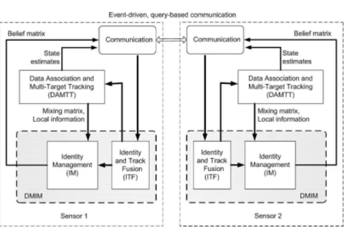
The overall architecture of DMTIM is shown in Fig. 3. DMTIM includes the Data Association and Multi-Target Tracking (DAMTT) module and the Distributed Multi-target Identity Management (DMIM) module which contains the Identity Management (IM) and Identity and Track Fusion
그림 3. DMTIM 시스템 구조 (두개의 센서인 경우) Fig. 3. An architecture of a distributed multi-target
tracking and identity management (DMTIM) system for a two-sensor example.
(ITF) submodules. At each sensor, the DAMTT module estimates the number of targets and tracks in its surveillance region using its local measurements and computes a mixing matrix and local information which are used by the IM module. A mixing matrix stores information about the interactions among targets while local information contains identity information about a target. A mixing matrix and local information are described in detail in [16]. Upon receiving a mixing matrix and local information, the IM module updates its belief matrix. Then the sensor transmits its updated belief matrix and estimated tracks to its neighboring sensors using the Communication unit.
In DMTIM, instead of sharing raw measurement data among neighboring sensors, the neighboring sensors share identity information in the form of a belief matrix and estimated tracks. As a result, we can reduce the overall communication load of the network. When the updated belief matrices and estimated tracks from neighboring sensors are available, the ITF module combines identity information and tracks, and maintains local consistency among sensors. For example, if the same target is seen by sensor 1 and sensor 2, then the ITF module makes sure that sensor 1 and sensor 2 share the same information about the target. The ITF module also combines multiple tracks of the same target into a single track and adds an entry for the identity of a new target into the belief matrix.
1. Example: Seven-Sensor Scenario
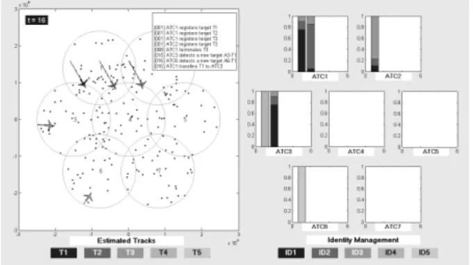
There are seven air traffic control radars (ATC1 through ATC7) and five aircraft (T1 through T5) as shown in Fig. 4, which represents the state of the system at simulation time t = 17. The left frame of Fig. 4 shows the position and heading of each aircraft along with sensing range (circle) of each sensor and measurements (dots). As the simulation time progresses, the left frame of Fig. 4 will show the estimated tracks and event logs. The right frame of Fig. 4 shows belief vectors of aircraft at each
그림 4. (시뮬레이션 시간 t = 16) 왼편 프레임은 추정 된 궤도와 사건기록을 보여줌. 초록 원은 각 센서의 감지 영역을 나타내고 검정 점들은 측 정값이다. 오른편 프레임은 각 센서가 가지고 있는 belief 벡터를 보여준다. 시뮬레이션 시간 t=15에 ATC3가 새로운 타켓을 발견한고 A3-T1 이라 라벨하고 ID4를 부여한다. 시뮬레이션 시 간 t=16에는 ATC6가 새로운 타겟을 발견하고 A6-T1이라 라벨하고 ID5를 부여한다. 같은 시 간에 ATC1이 T1을 ATC3에게 전달한다.
Fig. 4. (Simulation time t = 16) The left frame shows the estimated tracks and event logs. Circles and dots represent sensing ranges and measurements, respectively. The shade of aircraft corresponds the true identity based on the shade shown basow Estimated Tracks. The right frame shows the based on the s maintainn basoesponds the true shade of espondsgment of the bategraponrepresents an identity based on the shade shown basow Identity Management. At t = 15, ATC3 itso detects a new target and the target is labeled as A3-T1 and identity ID4 is assigned to this target. At t = 16, ATC6 detects a new target and the target is labeled as A6-T1 and identity ID5 is assigned to this target. At the same time, ATC1 transfers T1 to ATC3.
sensor. The order of belief vector is dictated by the order the target is registered to the corresponding sensor. Out of five targets, only three targets (T1, T2, and T3) are known to the system initially and the targets T4 and T5 are unknown to the system.
At time t = 1, targets T1, T2 and T3 are registered to ATC1 and target T3 is registered to ATC2. The identities ID1, ID2 and ID3 are associated to targets T1, T2 and T3, respectively. At t = 8, ATC1 terminates T3 since the target moves away from the sensing region of ATC1. At t = 15, ATC3 detects a new target and the target is labeled as A3-T1 and
identity ID4 is assigned to this target. At t = 16, ATC6 detects a new target and the target is labeled as A6-T1 and identity ID5 is assigned to this target.
At the same time, ATC1 transfers T1 to ATC3. See Fig. 4.
At t = 80, the belief matrix of ATC7 is
, (4) where the rows 1 through 5 of the belief matrix BATC7(80) correspond to identities ID1 through ID5 and the first and second columns of the belief matrix correspond to targets A3-T1 and T1, respectively.
At the same time, local information about target A3-T1 is obtained by ATC7 and target A3-T1 is now thought to have belief . This local information is incorporated according to the fusion algorithm described in [16]. First, a new matrix
′ is formed by replacing the column for target A3-T1 with local information, where
′
. (5) Since ′ is almost scalable, the scaled belief matrix is computed as:
″
. (6) The scaled belief matrix ″ decreases
그림 5. (t = 79) ATC7에 의해 belief matrix가 변경되기 전.
Fig. 5. (t = 79) Before the belief matrix update by ATC7.
그림 6 (t = 80) A3-T1에 대한 지역정보를 이용하여 belief matrix가 변경된 이후.
Fig. 6. (t = 80) The belief matrix is updated due to the local information about target A3-T1 obtained by ATC7.
entropy from 2.9091 to 2.3602. Hence, we assign
″ . See the updated belief matrix in Fig. 6 and compare it against Fig. 5.
Ⅳ. Camera Network Localization
The research in wireless sensor networks (WSNs) has traditionally focused on low-bandwidth sensors (e.g., acoustic, vibration, and infrared sensors) that limit the ability to identify complex, high-level physical phenomena. To address these limitations, there is a growing interest in camera sensor networks using low-power radios [18]. Camera sensor networks must operate in an uncontrolled environment without human intervention. In order to fully take advantage of the information from the network, it is important know the position of the cameras in the network as well as the orientation of their fields of view, i.e., localization. By localizing the cameras, we can perform better in-network image processing, scene analysis, data fusion, power hand-off, and surveillance. While there are localization methods for camera networks, they all make artificial requirements.
We removed these artificial requirements and developed a camera network localization method based on MCMCDA by associating tracks from multiple views[19]. The proposed method can be used
even when cameras are wide-baseline or have different photometric properties. The method can reliably compute the orientation of a camera's view and position only up to a scaling factor. We later removed this restriction by combining our technique with radio interferometry[20] to recover the exact orientation and position in [21].
Ⅴ. Multi-Sensor Fusion and Tracking
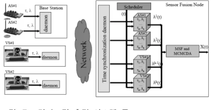
MCMCDA has been successfully applied to fuse audio and video sensor data for target tracking in [22]. The architecture of the system described in [22]
is shown in Fig. 7. The sensor network consists of audio sensors that perform beamforming and video sensors that detect moving objects. All nodes are time synchronized to allow sensor fusion. The sensor fusion node contains circular buffers that store timestamped measurements. A sensor fusion scheduler is triggered periodically and generates a fusion timestamp which is used to retrieve the sensor measurement values from the sensor buffers with timestamps closest to the generated fusion timestamp.
The retrieved sensor measurement values are then used for multimodal fusion, estimation, and tracking.
We briefly describe the main components of the system.
그림 7. 멀티모달 추적 시스템 구조
Fig. 7. Multimodal tracking system architecture.
1. Audio Beamforming
Beamforming can be used to determine the direction(s) of arrival and the location(s) of acoustic source(s)[23]. A typical delay-and-sum beamformer
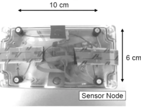
그림 8. 4개의 마이크가 장착된 센서 모듈 Fig. 8. Sensor node showing the microphones.
divides the sensing region into directions, or beams.
For each beam, assuming the source is located in that direction, the microphone signals are delayed according to the phase-shift and summed together into a composite signal. The square-sum of the composite signal, or the beam energy, is computed for each of the beams, and are collectively called the beamform. The beam with maximum energy indicates the direction of the acoustic source.
In our system, the audio sensor node is a MICAz mote with an onboard Xilinx XC3S1000 FPGA chip that is used to implement the beamformer. The board supports four independent analog channels. A small beamforming array of four microphones arranged in a 10 cm x 6 cm rectangle was placed on the sensor node, as shown in Fig. 8.
The sources are assumed to be on the same two-dimensional plane as the microphone array.
Thus, it is sufficient to perform planar beamforming by dissecting the angular space into equal angles, providing a resolution of degrees. In the experiments, the sensor boards were configured to perform simple delay-and-sum-type beamforming in real time with beams, at an angular resolution of 10 degrees per beam.
2. Motion Detection Using Video
Video tracking systems aim at detecting moving objects and track their movements in a complex environment. A simple approach to motion detection from video data is via frame differencing. It compares each incoming frame with a background model and
classifies the pixels of significant variation into the foreground. The foreground pixels are then processed for identification and tracking. We have implemented a motion detection algorithm using the background- foreground segmentation approach described in [24]
which is a based on an adaptive background mixture model and provides robust performance and low complexity in a wide range of situations. Our sensor fusion method utilizes only the angle of moving objects. Thus, we compute a simple detection function similar to the beam angle concept in audio beamforming. The detection function value for each beam direction is simply the number of foreground pixels in that direction. This detection function is similar to the horizontal intensity accumulation function (IAF) defined in [25]. In our experiments, we gathered video data of vehicles from multiple video sensors from an urban street setting. The data contained a number of real-life artifacts such as vacillating backgrounds, shadows, sunlight reflections and glint. The algorithm described above was not able to filter out such artifacts from the detections.
We implemented two post-processing filters to improve the detection performance to remove undesirable persistent background and sharp spikes caused by sunlight reflections and glint.
3. Evaluation
The deployment of the multi-modal target tracking system is shown in Fig. 9. We employ 6 audio sensors and 3 video sensors deployed on either side of a road. The complex urban street environment presents many challenges including gradual change of
그림 9. 실험 환경
Fig. 9. Experimental setup.
illumination, sunlight reflections from windows, glint due to cars, high visual clutter due to swaying trees, high background acoustic noise due to construction and acoustic multipath effects. The objective of the system is to detect and track vehicles using both audio and video under these conditions.
Sensor localization and calibration for both audio and video sensors is required. In our experimental setup, we manually placed the sensor nodes at marked locations and orientations. The audio sensors were placed on 1-meter high tripods to minimize audio clutter near the ground.
Table 1 presents the parameter values that we use in our tracking system. Sensor likelihood functions were calculated by discretizing the sensing region in specified cell-sized grid. The tracked vehicles were part of an uncontrolled experiment. The vehicles were traveling on the road at 15-30 mph.
In our simulations we experimented with six different approaches. We used audio-only, video-only and audio-video sensor observations for sensor fusion. For each of these data sets, the combined likelihood was computed either as the weighted sum or product of individual sensor likelihood functions (two fusion methods proposed in [22]).
The ground truth is estimated post-facto based on the video recording by a separate camera. The standalone ground truth camera was not part of any network, and had the sole responsibility of recording video. For evaluation of tracking accuracy, the center of mass of the vehicle is considered to be the true location.
We shortlisted 9 vehicle tracks where there was only a single target in the sensing region. The average duration of tracks was 3.75 sec with 2.75 sec minimum and 4.5 sec maximum. Fig. 10 shows
Number of beams in audio beamforming 36 Number of angles in video detection 160 Sensing region (meters) 35 x 20 Cell size (meters) 0.5 x 0.5
표 1. 실험에 사용된 함수 값
Table 1. Parameters used in experimental setup.
average tracking errors for all vehicle tracks for all target tracking approaches mentioned above. The missing bars indicate that the data association algorithm was not able to successfully estimate a track for the target. Fig. 11 averages tracking errors for all the tracks to compare different tracking approaches.
The audio and video modalities are able to track vehicles successfully, though they suffer from poor performance in the presence of high background noise and clutter. In general, audio sensors are able to track vehicles with good accuracy, but they suffer from high uncertainty and poor sensing range. As expected, fusing the two modalities gives better performance. There are some cases where the audio tracking performance is better than fusion. This is because of the poor performance of video tracking.
Video cameras were placed at an angle along the road to maximize coverage of the road. This makes video tracking very sensitive to camera calibration errors and camera placement. Also, an occasional obstruction in front of a camera confused the tracking algorithm, which would take a while to recover.
Fusion based on a product of likelihood functions gives better performance but it is more vulnerable to
그림 10. 추적 오차 (a) weighted sum. (b) product.
Fig. 10. Tracking errors (a) weighted sum, (b) product.
그림 11. 모든 track에 대한 평균 오차 Fig. 11. Average tracking errors for all tracks.
sensor conflict and errors in sensor calibration, etc.
The weighted-sum approach is more robust to conflicts and sensor errors, but it suffers from high uncertainty. The average tracking error of 2 meters is reasonable considering the fact that a vehicle is not a point source, and the cell size used in the audio-video fusion experiment is 0.5 meters.
Ⅵ. Conclusions
In this paper, we have described the Bayesian formulation of data association and applications of data association in intelligent systems, identity management for air traffic control, camera network localization, and multi-sensor fusion. Since data association is a fundamental problem in intelligent systems, we envision that there will be more applications of data association in intelligent systems.
References
[1] D. Reid, An algorithm for tracking multiple targets, IEEE Trans. Automatic Control 24 (6) (1979) 843–854.
[2] Y. Bar-Shalom, T. Fortmann, Tracking and Data Association, Academic Press, San Diego, CA, 1988.
[3] S. Oh, S. Russell, S. Sastry, Markov chain Monte Carlo data association for multi-target tracking, IEEE Trans. Automatic Control 54 (3) (2009) 481–497.
[4] I. Cox, A review of statistical data association
techniques for motion correspondence, International Journal of Computer Vision 10 (1) (1993) 53–66.
[5] I. Cox, S. Hingorani, An efficient implementation of Reid’'s multiple hypothesis tracking algorithm and its evaluation for the purpose of visual tracking, IEEE Trans. Pattern Analysis and Machine Intelligence 18 (2) (1996) 138–150.
[6] D. Forsyth, J. Ponce, Computer Vision: A Modern Approach, Prentice-Hall, 2003.
[7] S. Thrun,W. Burgard, D. Fox, Probabilistic Robotics, Intelligent Robotics and Autonomous Agents, MIT Press, 2005.
[8] U. Frese, A discussion of simultaneous localization and mapping, Autonomous Robots 20 (1) (2006) 25–42.
[9] S. Oh, L. Schenato, P. Chen, S. Sastry, Tracking and coordination of multiple agents using sensor networks: System design, algorithms and experiments, Proceedings of the IEEE 95 (1) (2007) 234–254.
[10] H. Pasula, B. Marthi, B. Milch, S. Russell, I.
Shpitser, Identity uncertainty and citation matching, in: Advances in Neural Information Processing Systems 15, MIT Press, 2003.
[11] G. Cybenko, V. Berk, V. Crespi, R. Gray, G.
Jiang, An overview of process query systems, in: Proc. of SPIE Vol. 5403, Sensors, and Command, Control, Communications, and Intelligence (C3I) Technologies for Homeland Security and Homeland Defense III, Orlando, FL, 2004.
[12] H. Pasula, S. J. Russell, M. Ostland, Y. Ritov, Tracking many objects with many sensors, in:
Proc. of the International Joint Conference on Artificial Intelligence, Stockholm, 1999.
[13] T. Kurien, Issues in the design of practical multitarget tracking algorithms, in: Y.
Bar-Shalom (Ed.), Multitarget-Multisensor Tracking: Advanced Applications, Artech House, Norwood, MA, 1990.
[14] A. Poore, Multidimensional assignment and multitarget tracking, in: I. J. Cox, P. Hansen, B.
Julesz (Eds.), Partitioning Data Sets, American Mathematical Society, 1995, pp. 169–196.
[15] I. Hwang, K. Roy, H. Balakrishnan, C. Tomlin, A distributed multipletarget identity management algorithm in sensor networks, in: Proc. of the 43rd IEEE Conference on Decision and Control, Bahamas, 2004.
[16] S. Oh, I. Hwang, S. Sastry, Distributed
저 자 소 개 오 성 회(평생회원)
1995년 UC Berkeley 전기컴퓨터공학 학사 2003년 UC Berkeley 전기컴퓨터공학 석사 2006년 UC Berkeley 전기컴퓨터공학 박사 1995년~1998년 Design Engineer, Intel Corp.
1998년~2000년 Senior Engineer, Synopsys, Inc.
2007년 Postdoctoral Researcher, UC Berkeley 2007년~2009년 Univ. of California, Merced
조교수
2009년~현재 서울대학교 전기·정보공학부 조교수
<주관심분야 : cyber-physical systems, wireless sensor networks, robotics, machine learning>
multi-target tracking and identity management, Journal of Guidance, Control, and Dynamics 31 (1) (2008) 12–29.
[17] I. Hwang, H. Balakrishnan, K. Roy, C. Tomlin, Multiple-target tracking and identity management with application to aircraft tracking, AIAA Journal of Guidance, Control and Dynamics.
[18] P.W.-C. Chen, P. Ahammad, C. Boyer, S.-I.
Huang, L. Lin, E. J. Lobaton, M. L. Meingast, S.
Oh, S. Wang, P. Yan, A. Yang, C. Yeo, L.-C.
Chang, D. Tygar, S. S. Sastry, CITRIC: A low-bandwidth wireless camera network platform, in: Proc. of the ACM/IEEE International Conference on Distributed Smart Cameras, Stanford University, CA, 2008.
[19] M. Meingast, S. Oh, S. Sastry, Automatic camera network localization using object image tracks, in: Proc. of the IEEE International Conference on Computer Vision Workshop on Visual Representations and Modeling of Large-scale environments, Rio de Janeiro, Brazil, 2007.
[20] M. Maroti, B. Kusy, G. Balogh, P. Volgyesi, A.
Nadas, K. Molnar, S. Dora, A. Ledeczi, Radio interferometric geolocation, in: Proc. of ACM SenSys, 2005.
[21] M. Meingast, M. Kushwaha, S. Oh, X.
Koutsoukos, A. Ledeczi, S. Sastry, Fusion-based localization for a heterogeneous camera network, in: Proc. of the ACM/IEEE International Conference on Distributed Smart Cameras, Stanford University, CA, 2008.
[22] M. Kushwaha, S. Oh, I. Amundson, X.
Koutsoukos, A. Ledeczi, Target tracking in heterogeneous sensor networks using audio and video sensor fusion, in: Proc. of the IEEE International Conference on Multisensor Fusion and Integration for Intelligent Systems, Seoul, Korea, 2008.
[23] J. Chen, L. Yip, J. Elson, H. Wang, D. Maniezzo, R. Hudson, K. Yao, D. Estrin, Coherent acoustic array processing and localization on wireless sensor networks, in: Proceedings of the IEEE, Vol. 91, 2003, pp. 1154–1162.
[24] P. KaewTraKulPong, R. B. Jeremy, An improved adaptive background mixture model for realtime tracking with shadow detection, in: Workshop on Advanced Video Based Surveillance Systems (AVBS), 2001.
[25] S. Karimi-Ashtiani, C. C. J. Kuo, Automatic real-time moving target detection from infrared video, in: International Conference on Intelligent Information Hiding and Multimedia Signal Processing (IIH-MSP’'06), 2006.
[26] Y. H. Jung, H, S. Shin, Suboptimal Detection Thresholds for Tracking in Clutter, IEEK, vol.
39-SC, no. 2, pp. 92-97, 2002.